ssts.nk
set cut_paste_input [stack 0]
version 11.0 v2
push $cut_paste_input
Group {
name SSTS_Red2
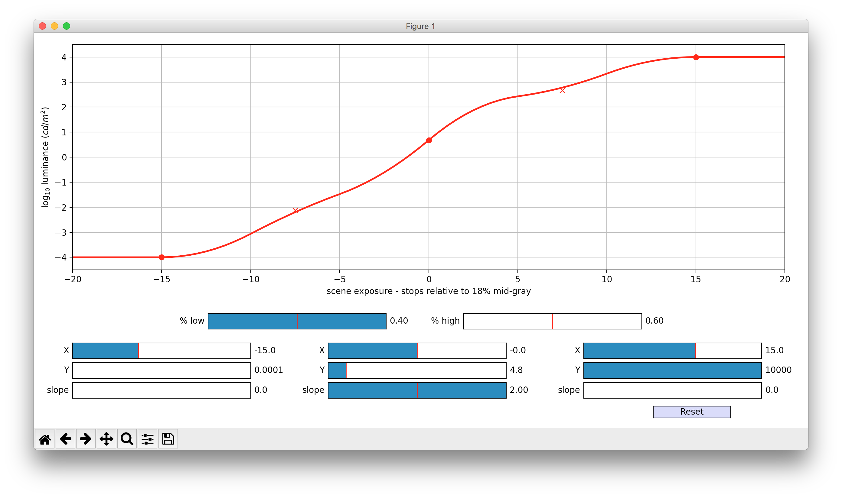
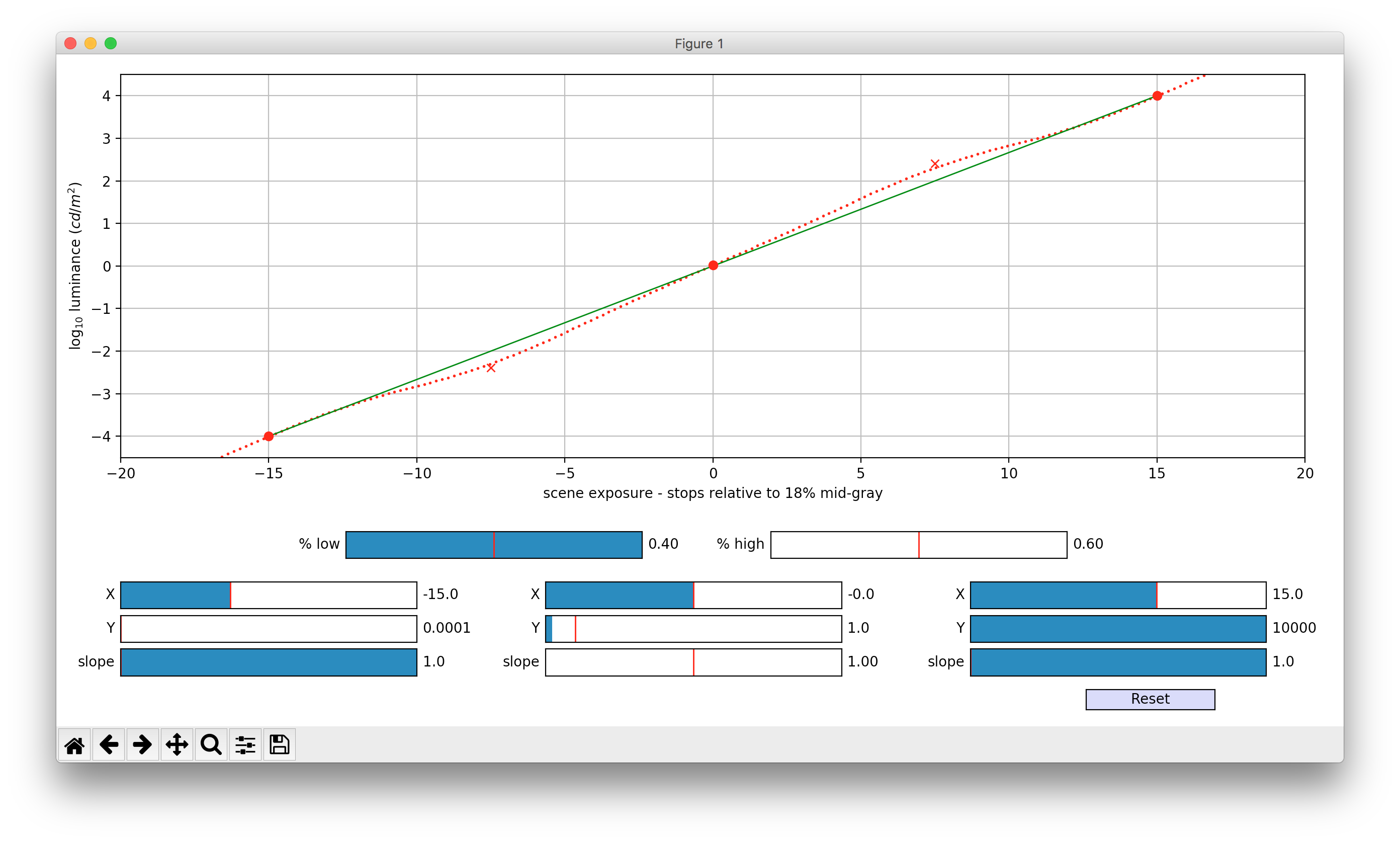
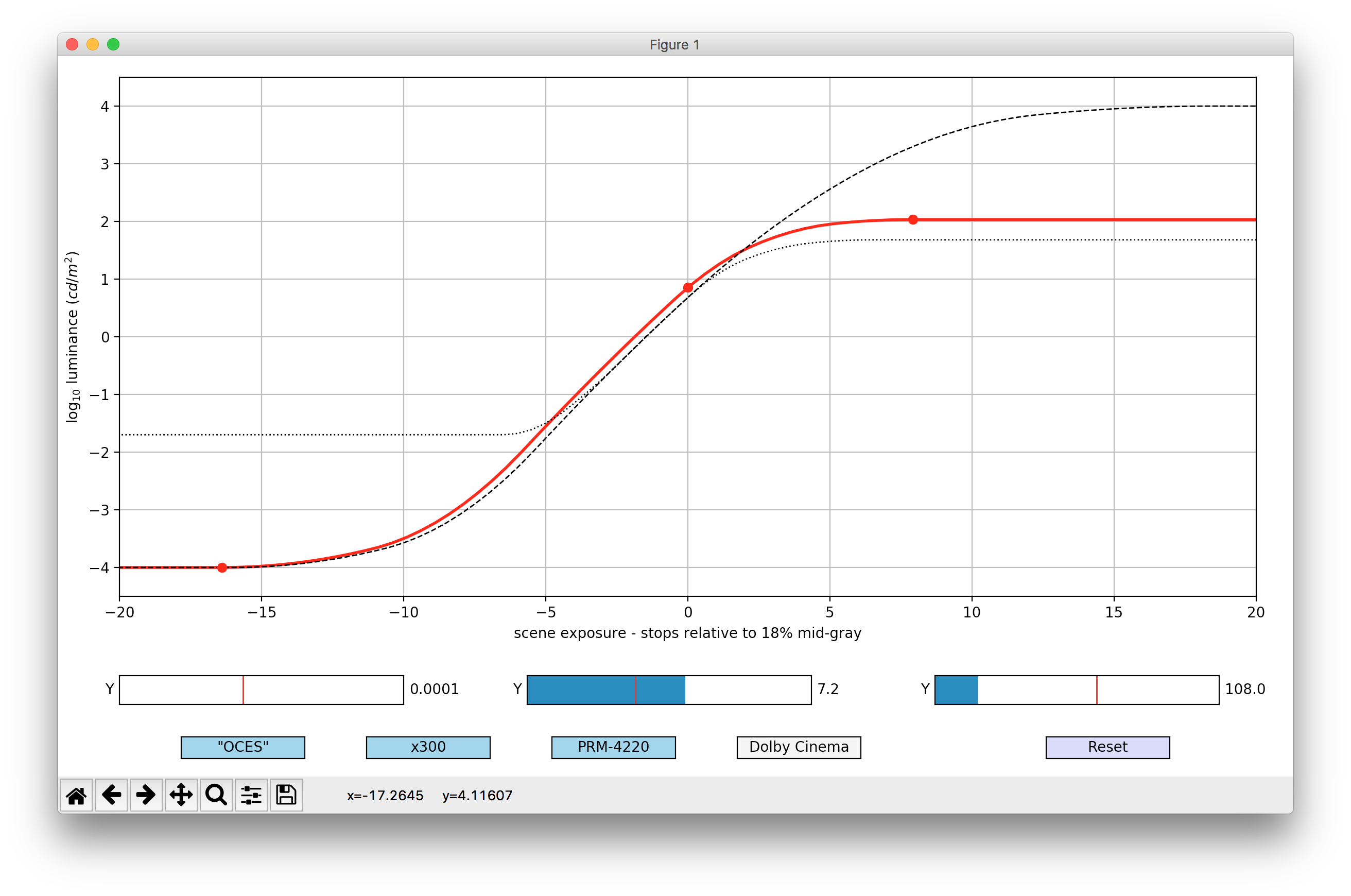
knobChanged "\nnode = nuke.thisNode()\nknob = nuke.thisKnob()\nname = knob.name()\n\nswitches = \['calcMin', 'calcMax', 'calcPctLow', 'calcPctHigh']\nsstsparms = \['min', 'mid', 'max', 'pctLow', 'pctHigh']\nothers = \['presets', 'inv', 'channel']\n\n\n\n\nif name not in (switches + others):\n pass\n\nelse: \n value = knob.getValue()\n if name == 'channel':\n\n def setcolor(dark, light):\n inverse = node\['inv'].getValue()\n if inverse < 1.0:\n node\['tile_color'].setValue(dark)\n node\['note_font_color'].setValue(light)\n else:\n node\['tile_color'].setValue(light)\n node\['note_font_color'].setValue(dark)\n rgb_hex = lambda rgb: int('%02x%02x%02x%02x' %\n (255*rgb\[0], 255*rgb\[1], 255*rgb\[2],1), 16)\n c = node\['channel'].value()\n\n if c == 'Red':\n pink = rgb_hex((0.95, 0.75, 0.75))\n red = rgb_hex((0.5, 0., 0.))\n setcolor(red, pink)\n elif c == 'Green':\n mint = rgb_hex((0.75, 0.95, 0.75))\n green = rgb_hex((0., 0.3, 0.))\n setcolor(green, mint)\n else:\n sky = rgb_hex((0.75, 0.75, 0.95))\n blue = rgb_hex((0., 0., 3.))\n setcolor(blue, sky)\n\n elif name == 'inv':\n oldtile = int(node\['tile_color'].getValue())\n oldnote = int(node\['note_font_color'].getValue())\n node\['tile_color'].setValue(oldnote)\n node\['note_font_color'].setValue(oldtile)\n\n\n\n elif name in switches:\n\n defaults = \{\n 'min' : \"clamp(minLum, pow(10,lumLow.x), pow(10,lumLow.y))\",\n 'max' : \"clamp(maxLum, pow(10,lumHigh.x), pow(10,lumHigh.y))\"\n \}\n switchexp = lambda x: node\[x].setExpression(exprs\[x],0) if value == 1.0 else node\[x].clearAnimated()\n exprs = \{\n 'min' : \"\"\"\n pow(2, (\n (log(\n (pow(2, lerp(lumLow.x, stopsLow.x, lumLow.y, stopsLow.y, log10(min.y))) * 0.18))\n /log(2)) \n - expShift))\n \"\"\",\n 'max' : \"\"\"\n pow(2, (\n (log(\n (pow(2, lerp(lumHigh.x, stopsHigh.x, lumHigh.y, stopsHigh.y, log10(max.y)))* 0.18))\n /log(2))\n - expShift))\n \"\"\",\n 'pctLow' : \"\"\"\n lerp(\n stopsLow.x,\n pctsLow.x,\n stopsLow.y,\n pctsLow.y,\n (log(min.x/0.18)/log(2))\n )\n\n \"\"\",\n 'pctHigh' : \"\"\"\n lerp(\n stopsHigh.x,\n pctsHigh.x,\n stopsHigh.y,\n pctsHigh.y,\n (log(max.x/0.18)/log(2))\n )\n \"\"\"\}\n if name == 'calcMin':\n switchexp('min')\n elif name == 'calcMax':\n switchexp('max')\n elif name == 'calcPctLow':\n switchexp('pctLow')\n elif name == 'calcPctHigh':\n switchexp('pctHigh')\n\n elif name == 'presets':\n\n presets = \{\n 'OCES' : (0.0001, 4.8, 10000.),\n 'Sony BVM-X300' : (0.0001, 10., 1000.),\n 'Dolby PRM-4220' : (0.005, 10., 600.),\n 'Dolby Pulsar' : (0.005, 15., 4000.),\n 'Dolby Cinema' : (0.0001, 7.2, 108.),\n 'Standard Cinema' : (0.02, 4.8, 48.),\n \}\n\n p = node\['presets'].value()\n if p in presets.keys():\n node\['mid'].setValue(presets\[p]\[1], 1)\n node\['min'].setValue(presets\[p]\[0], 1)\n node\['max'].setValue(presets\[p]\[2], 1)\n for k in \['min', 'mid', 'max']:\n node\[k].setEnabled(False)\n else:\n for k in sstsparms:\n node\[k].setEnabled(True)\n\n\n\n"
tile_color 0x7f000001
gl_color 0xffffffff
label "\[value min.y]\n\[value max.y]\n\[? \[numvalue presets]==0 \"\" \[value presets]]\n\[expr \[value inv]?\"inverse\":\"\"]"
note_font Verdana
This file has been truncated. show original