ACES 2.0 CAM DRT Development

That’s an interesting question. Since Resolve on iPad doesn’t have separate user and system LUT folders, like the Mac version does, it is not obvious where custom IDT/ODT DCTLs would go. I’ll see if I can find out.

In the meantime, you can use them as normal DCTLs by removing the first line:

DEFINE_ACES_PARAM(IS_PARAMETRIC_ACES_TRANSFORM: 0)

I just tested on my iPad Pro and that seems to work.

Thank you Nick.
They do indeed work that way.
Now to play around a bit.

FYI, Reference mode turns off local dimming. So you end up with a standard 1000:1 LCD display.

2 Likes

Is that definitely the case? I can put up a 1000 nit patch and still measure absolute black elsewhere on the screen.

I only have an X-Rite i1Display3, but I read zero luminance as far as that can tell.

Daniele et all,
Seems to do more than just that according to Apple:

When using “B: Stock DaVinci YRGB project with manual ACES node” as suggested in:

When setting the Output Color Space to Rec.709 the display looks to be a maximum of 100 nits and the ACES2 Candidate CAMDRT rev027 Rec709 looks pretty close to that on my SDR computer with same settings with an ASUS ProArt PA329C 32" 16:9 4K HDR IPS Display at Rec709.

When setting the Output Color space to Rec.2100 ST2084 the display looks to be a maximum of 1000 nits with the ACES2 Candidate CAMDRT rev027 Rec2100 (P3D65 1000nit Limited) and looks pretty close to that on my HDR computer with same settings with a LG C8PUA 55" 4K HDR OLED TV.

Also when using the ACES2 Candidate CAMDRT rev027 Rec2100 (Rec709 sim), (on the iPad), the maximum white of an image looks to be 100nits and very close to that on both the SDR computer and the iPad with Rec.709 settings and ODT (and on the HDR computer set to SDR.)

I am confident that the differences are due to calibration (or lack thereof) and could easily be corrected. In fact, I might even guess that my i1 Display Pro sensor might be more inaccurate than the new iPad Pro.

I also add that the iPad Pro seems to give a better image at full screen than in the small Resolve color page window, but they are close and the Resolve window on the iPad could be used for rough grading of either SDR or HDR. Of course, I would always recommend checking with a fully calibrated pro monitor for any important work. Even so it is nice the be able to put the three screens next to each other.

I made pull request for @alexfry for v28, also available in my fork . It brings the following:

  • Adds path-to-black to reduce clipping in the shadows and reduce excessive colorfulness in the shadows. Chroma compression desmos plot.

  • The old per-hue angle compression in chroma compression is now replaced with a hue-dependent curve. This is simpler, smoother, and more elegant implementation. The curve has less compression in yellows to improve inversion compared to previous version. Hue dependent curve desmos plot.

  • Adds lightness based compression to gamut mapper. Darker colors can be compressed more than lighter colors. Highlights already have strong compression (chroma compression step) but shadows aren’t compressed nearly as much; more darker colors are out-of-gamut than lighter colors. This reduces clipping in shadows. GUI now has min limit and max limit that can be adjusted. If both min and max are same value, it behaves same way as previous version.

  • Adds lightness based focus point adjustment to gamut mapper. This can make the projection to focus point for darker colors slightly shallower, and for lighter colors slightly steeper. GUI now has min distance and max distance that can be adjusted. If both min and max are same value, it behaves same way as previous version.

  • Removes the old highlight desat mode.

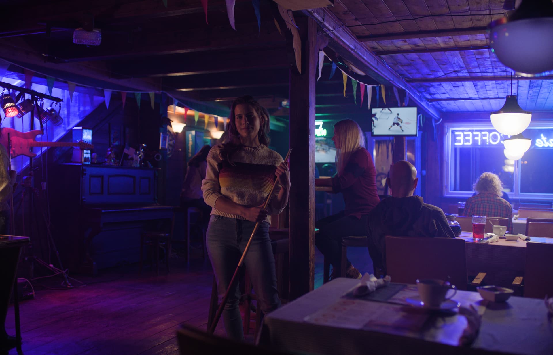
The rendering hasn’t changed much but darker colors can render slightly darker than before because noise is now less colorful. HDR had always slightly less saturated shadows than SDR so the SDR/HDR match should be a bit closer in this version. Reds are slightly darker in SDR because of the gamut mapper changes listed above. SDR reds match a bit better to HDR reds (ie. darker) but much room for improvement.

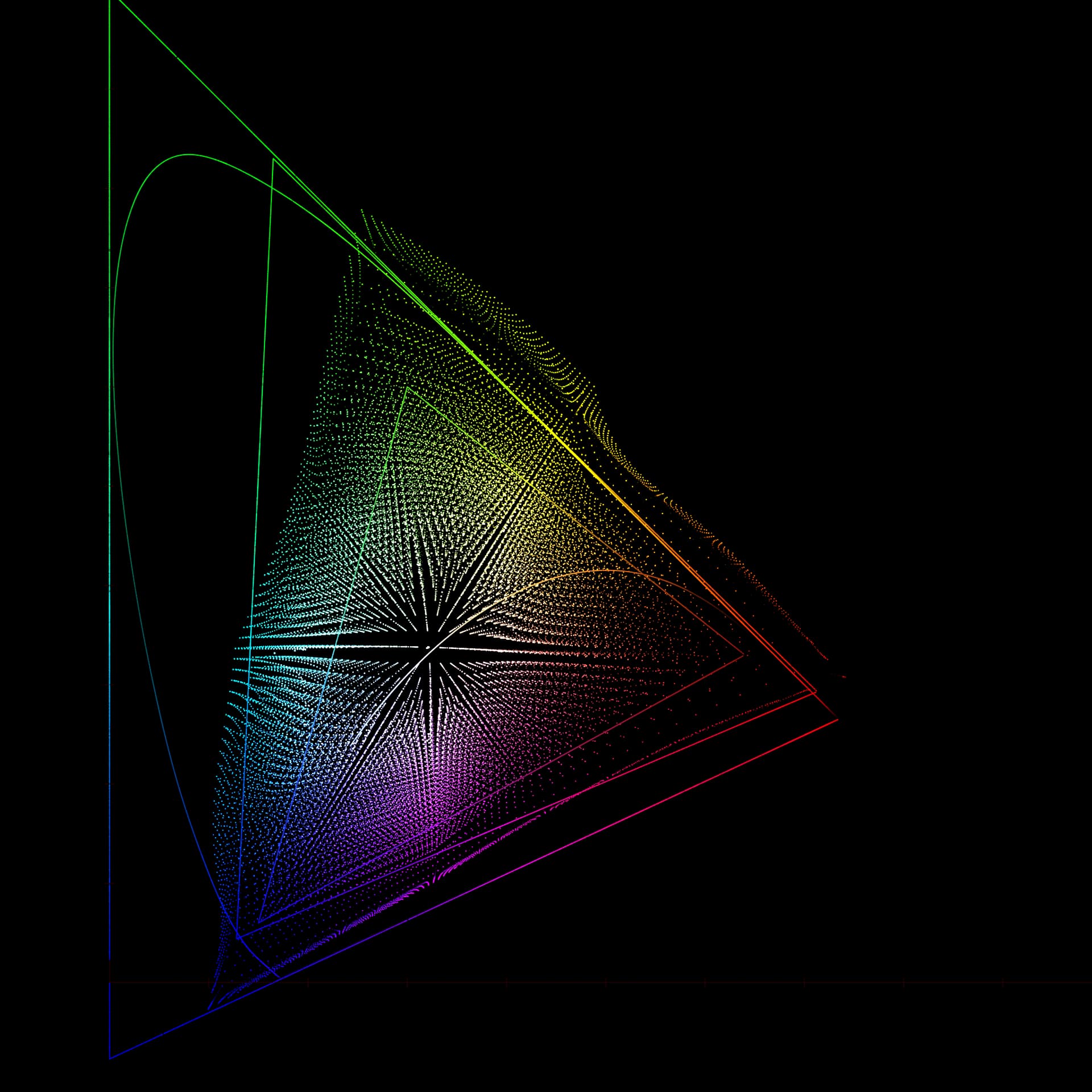
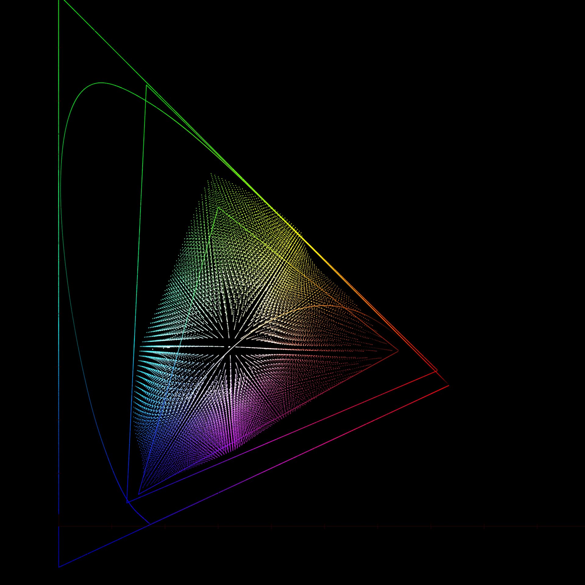
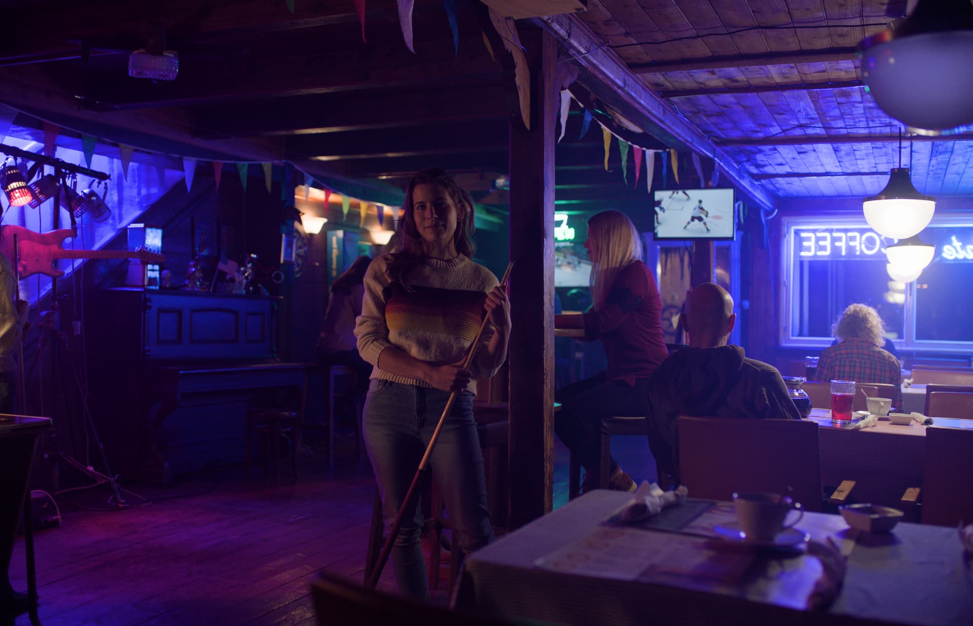
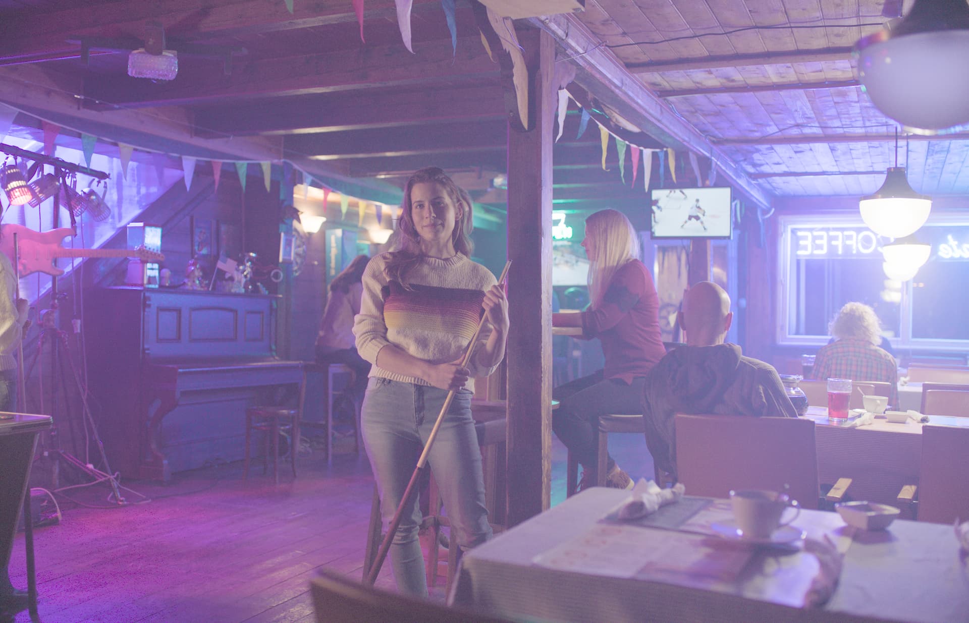
Following images are v28 first, v27 second. Some images are gamma up 5 to show what happens in the shadows now.


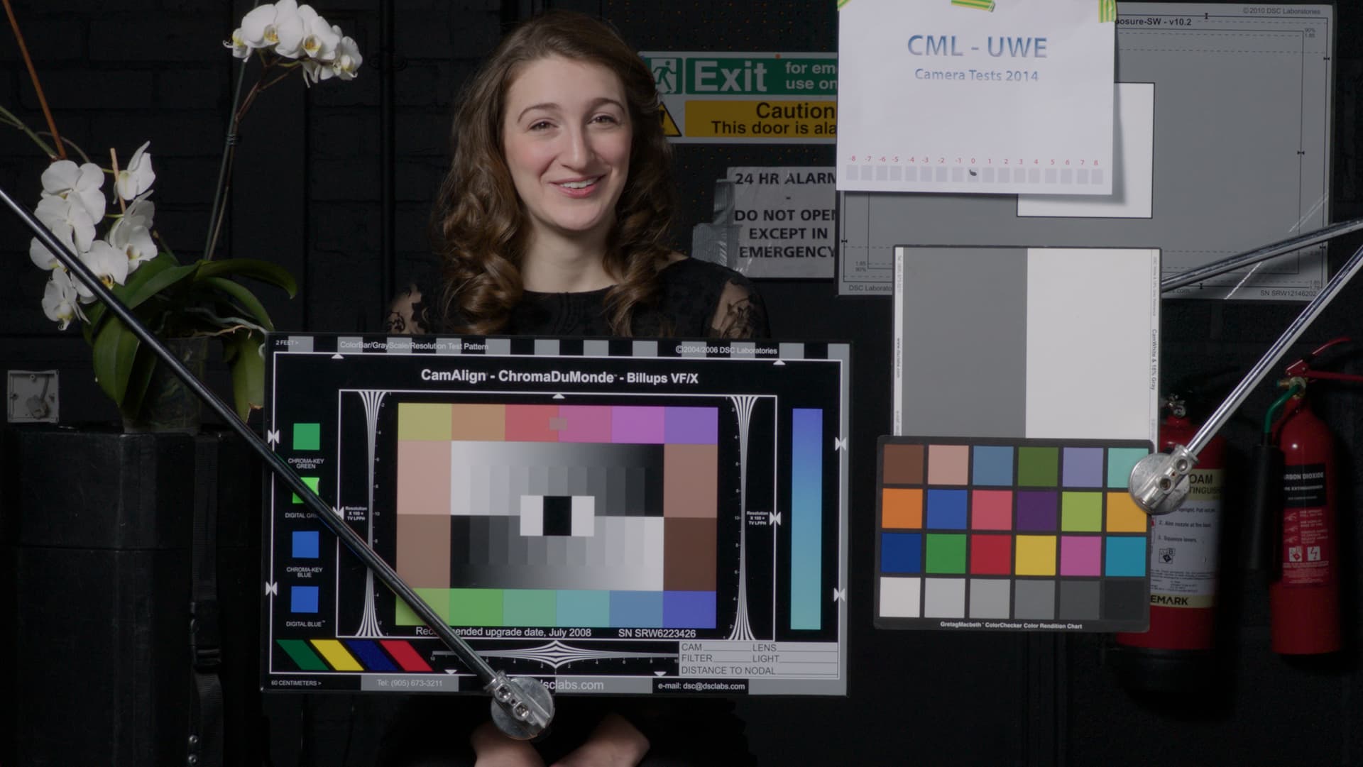
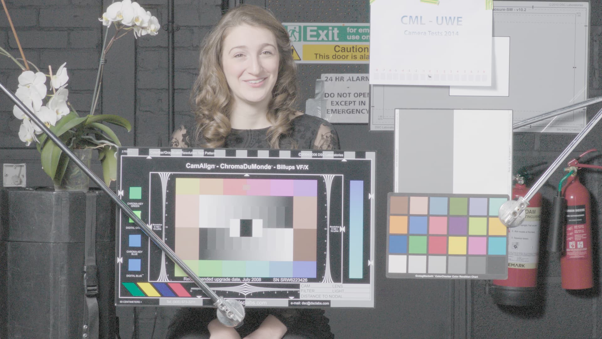
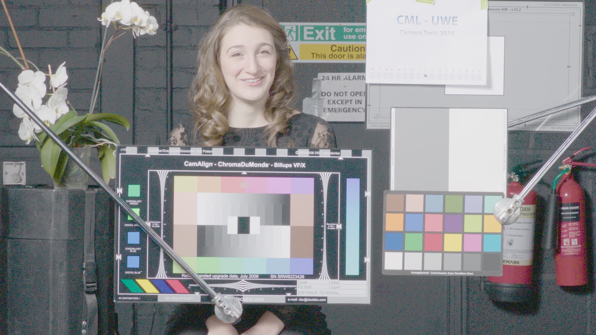
In the last meeting I think Alex was showing the inverse without the gamut mapper enabled. Here’s what v28 inverse is with both gamut mapper enabled and disabled (Rec.709 cube):


1 Like

I think so, at least in SDR.
In HDR I am not 100% sure yet what is going on.

2 Likes

v28 looks very nice (to my eyes at least).

The inverse is good, but not perfect. A Rec.709 cube run backwards then forwards through the DRT loses a little bit around the edges:

Hmm… I think that’s a bug. The inverse was clean in v27, I believe. Might be the gamut mapper changes in v28 at fault.

The gamut mapper will have biggest impact for inverse anyway, so rather than tweaking the current gamut mapper (like I did in v28) it would better to have a gamut approximation based implementation, and tweak that. I’m assuming the current implementation, which uses LUT for finding the cusp and iterative approach to find the boundary, isn’t appropriate for final implementation.

But the one that goes outside the spectral locus is the one with the gamut mapper enabled, which is what @alexfry showed. That makes sense, because in an inverse, the gamut compressor becomes a gamut expander.

Actually I can’t reproduce this. Did you by any chance have RGC enabled?


The v27 with gamut mapper version is even more outside. Here’s v27 with and without gamut mapper (as can be seen v28 improves inverse, v27 added more compression to deal with shadow clipping but it was meant to be temporary solution, which v28 now addresses):


No. Just v28, settings as per your repo in both directions.

I am inverting from Rec.709 / BT.1886. If I use a Rec.709 / linear inverse it appears to fill the cube, as you show. For inverting real world display-referred imagery, I would say that the 2.4 gamma needs to be included in both directions.

EDIT: sRGB in both directions comes closer to filling the cube. I’m assuming that a small inaccuracy in inversion is exaggerated by the inverse 2.4 gamma. Less so by the linear portion at the bottom of sRGB.

Using the Python implementation with compress mode from @Thomas_Mansencal’s Colab (with a small tweak of the compress/decompress fuctions to trap for divide by zero when x=y=z) I see the same result with a BT.1886 → JMh → BT.1886 round trip. Using just the eight corners of the cube (i.e. primaries, secondaries, black and white) after the round trip I get:

[[[[-0.0000000000 0.0000000000 0.0000000000]
   [0.0365082030 0.0368818295 0.9995565545]]

  [[0.0397139681 0.9998362401 0.0348177461]
   [0.0150639031 1.0000119030 1.0000046571]]]


 [[[0.9992951472 0.0354635798 0.0291468397]
   [0.9999506298 0.0253964397 0.9999180909]]

  [[0.9998752347 0.9999066957 0.0383670810]
   [1.0000062083 1.0000225205 1.0000066041]]]]

0.0397139681 is 10-bit code value 41, which is quite a significant difference from zero.

A post was split to a new topic: Issues using Oklab transform in Nuke

It does seem to be clipping of fully saturated colours, rather than distorting of the cube. If I use a cube of 0.1 and 0.9 values instead of 0 and 1, I get:

[[[[0.1000006208 0.1000022520 0.1000006604]
   [0.1001876482 0.0999380216 0.9000013549]]

  [[0.1000006208 0.9000151462 0.1000969808]
   [0.1001876482 0.9000121840 0.9000058020]]]


 [[[0.8999969470 0.1001772577 0.1000037330]
   [0.9000055875 0.1001131844 0.9000014967]]

  [[0.8999969470 0.9000232306 0.1001000493]
   [0.9000055875 0.9000202684 0.9000059437]]]]

It may not be exact, but it’s close enough to be down to calculation rounding errors. And the round trip difference is less than one 12-bit code value.

I was also looking again at the Blink code, when did the spow function get changed from mirroring to clamping? Was that something @matthias.scharfenber did back in the ZCAM version? We need to be careful of things which were done to fix an issue which may not necessarily still be the case.

Clamping may make sense in many cases in a DRT (we don’t want erroneous “negative light” affecting the result) but might it be better to clamp pixels with negative luminance on input, but retain other negatives which might be out of gamut values?

I believe the spow() has been that way for a very long time. The commented-out code was added later, and never taken into use.

@Thomas_Mansencal ’s Python implementation uses Colour’s built in spow which I believe defaults to mirroring.

I’ve done some testing on the path of the cusp, again using @Thomas_Mansencal 's Python. I’m not sure that my Python and Blink XYZ <-> JMh conversions give identical results, but this is a test of principle more than anything else.

cusp

The path of the cusp (Rec.709 cube in this case) is very peculiarly shaped. I think we would need to accept a very crude match if we wanted to use a function to approximate it.

Although I suppose the six obvious cusps in the paths are the primaries and secondaries, so perhaps just joining those six points with suitable curves might be reasonable. The path of the cusp in J could even be fairly reasonable approximated with six straight lines.

2 Likes

I think a smooth approximation of that M path is not impossible.

As far as the cusp J goes, we might not even need that. If you look at the current mapper it doesn’t really use the cusp J directly. The focus point J is always a blend of middle gray and the cusp J. And that choice of blend is entirely arbitrary (it’s set to 0.5 at the moment, half way between middle gray and the cusp J). So we could just have a smooth curve that gives us directly J we like.

When I was testing this, I found that having the blend closer to cusp J for secondary colors and closer to middle gray for primary colors, produced the best mapping to my eye. Current 0.5 blend darkens yellows and cyans maybe a bit too much as their cusp J is very high, as can be seen from the plot. Middle gray is under any cusp J.

But can “picking a curve we like” be generalised to all display targets? Or do you you think the same J curve could be applied to all, just scaled with peak white?