There’s been recently some discussion on how the ACES2 DRT uses the AP1 gamut cusp value in the chroma compression, and might there be a way to change it so that the AP1 cusp table would no longer be needed. Many many months ago I kind of promised I was going to approximate the AP1 gamut cusp so that we could use the approximation instead which would eliminate the table. But I never got around doing that. Until now.
This post is meant to give some more context on how the AP1 cusp value is being used, and why, as well as to show the experiment.
What is the AP1 cusp used for in ACES2 chroma compression?
It is used as a normalization value in what’s called a “normalization step” in the chroma compression. That step simply divides the colorfulness correlate M with a value before compressing the M.
The normalization affects the aggressiveness of the compression for a given hue. That’s because the value is hue dependent, and because larger values will push larger M values deeper into the heart of the compression curve (which compresses smaller M values more than larger ones). If one wanted to compress some particular hue more aggressively the normalization value for that hue could be increased. In other words, the normalization has a strong impact on the “look”.
But the normalization value itself is kind of meaningless. One could come up with any random value and be perfectly happy with the “look”. However, it should be picked by keeping certain things in mind.
The normalization value should be anchored on something that doesn’t change when the transform changes. It wouldn’t be a good idea for example to use the display gamut cusp J or M because the rendering would then change by simply changing the gamut from Rec.709 to P3, all else being equal. It also wouldn’t be a good idea to use the input J or input M as that would make the rendering different for each input. In both these cases we want the rendering to not change.
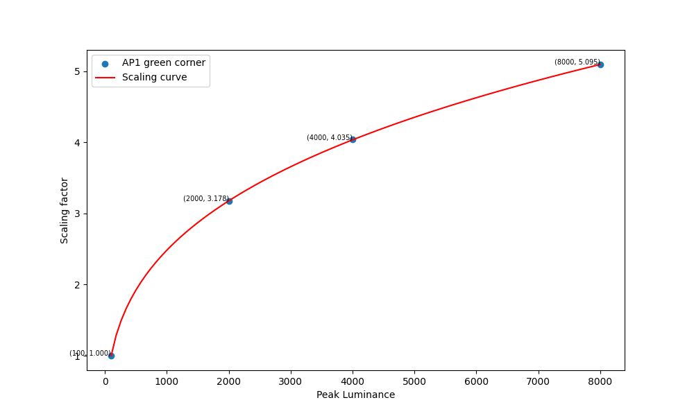
When the display peak luminance changes the model space scales. The JMh space becomes bigger with higher peak luminance. It scales up with the so called “model gamma”, or the {\frac{1}{cz}} exponent in the Hellwig2022 model. This means that the normalization value has to scale up as well so that it ends up doing similar thing in similar location in the bigger space. That’s why a constant value as a normalization value doesn’t work. It’s also the reason why the reachM (the M at limitJmax in AP1) is not a good normalization value. While that does scale up with the peak luminance, it ends up being in a very different location for different displays, being the peak value. A good normalization value stays relatively in the same location when the space scales up.
This all has to do with the appearance match between different displays. We want the appearance of the rendering essentially to not change even though the display changes. So for ACES2 DRT, the rendering space, AP1 cusp, is a convenient value to use for the normalization.
The value doesn’t have to be exact. It’s not like the reach M value that needs to be precise for the inverse to work. The normalization value doesn’t have to be precise.
The experiment with ACES2 DRT with AP1 cusp hue dependent curve
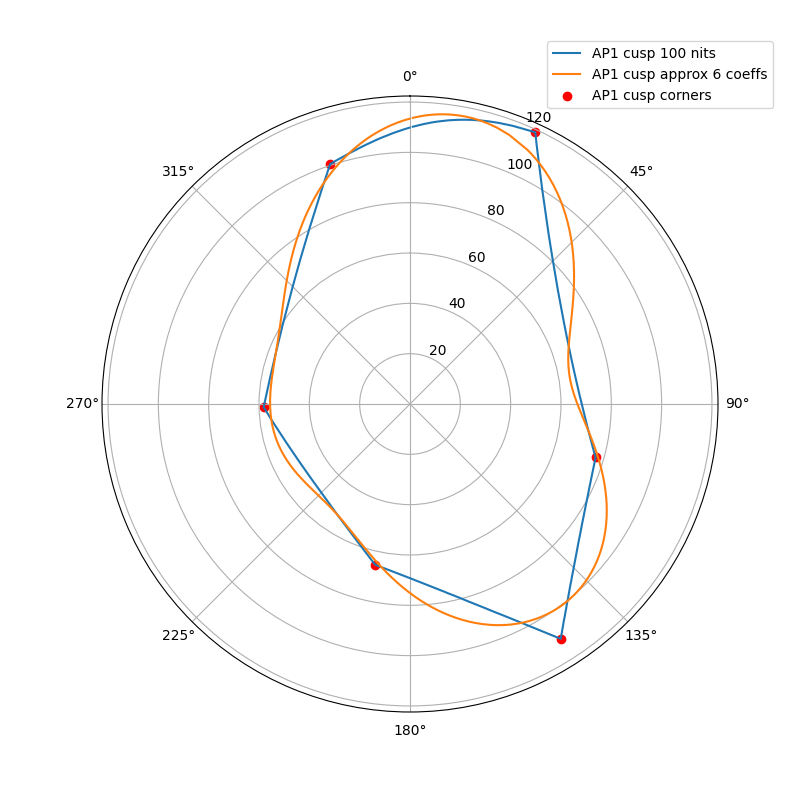
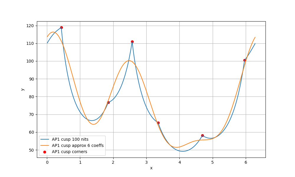
I wanted to experiment with a ballpark approximation of AP1 cusp and use that in place of the actual cusp in chroma compression to see how close I could get the look and the behavior to match the ACES2 DRT. The approximation is a hue dependent trigonometric function (with 6 cos/sin coefficients). The curve will automatically scale based on the peak luminance.
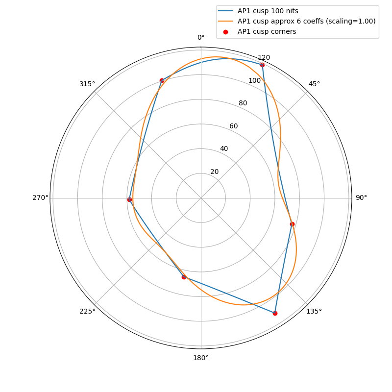
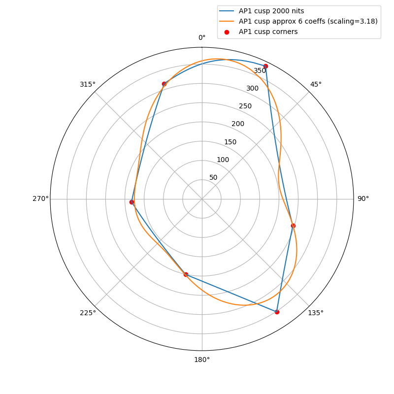
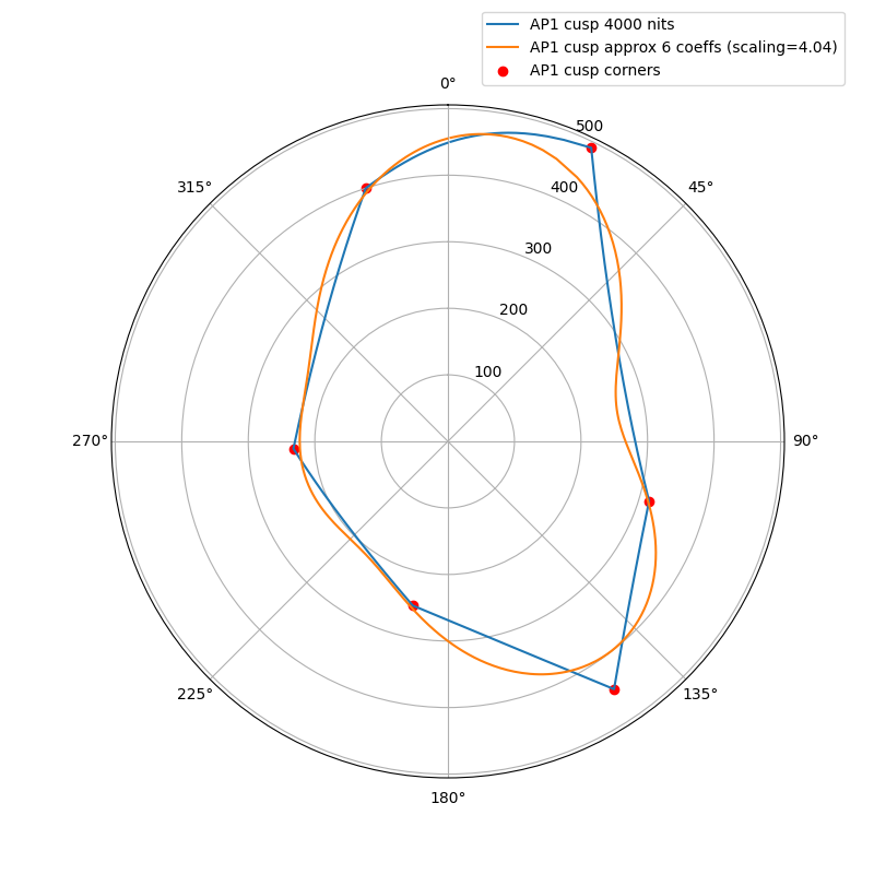
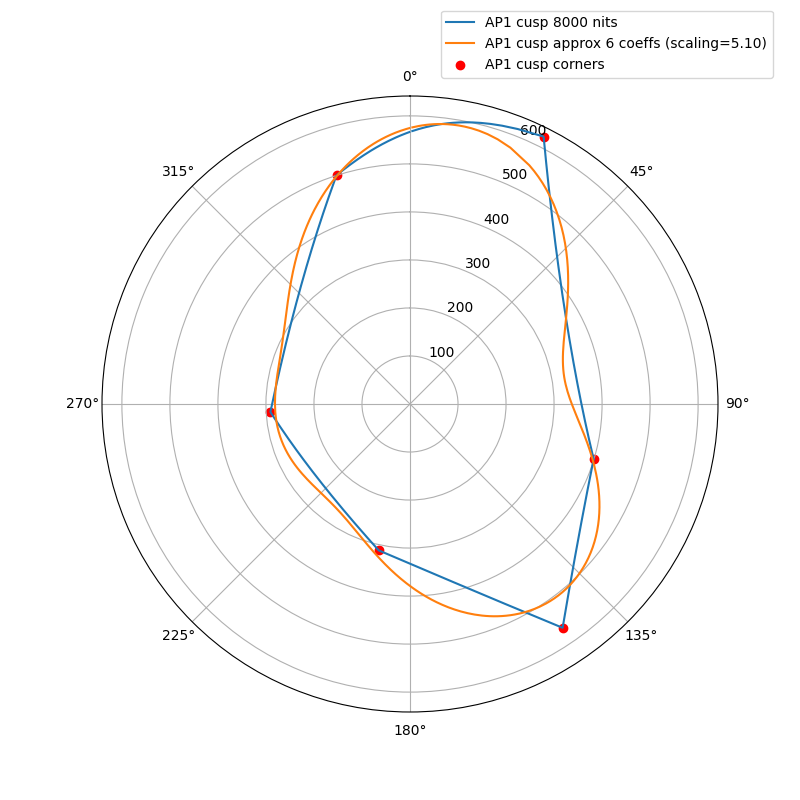
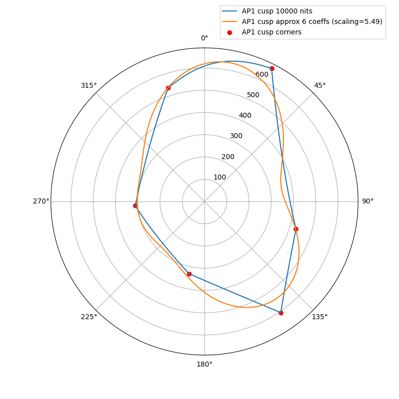
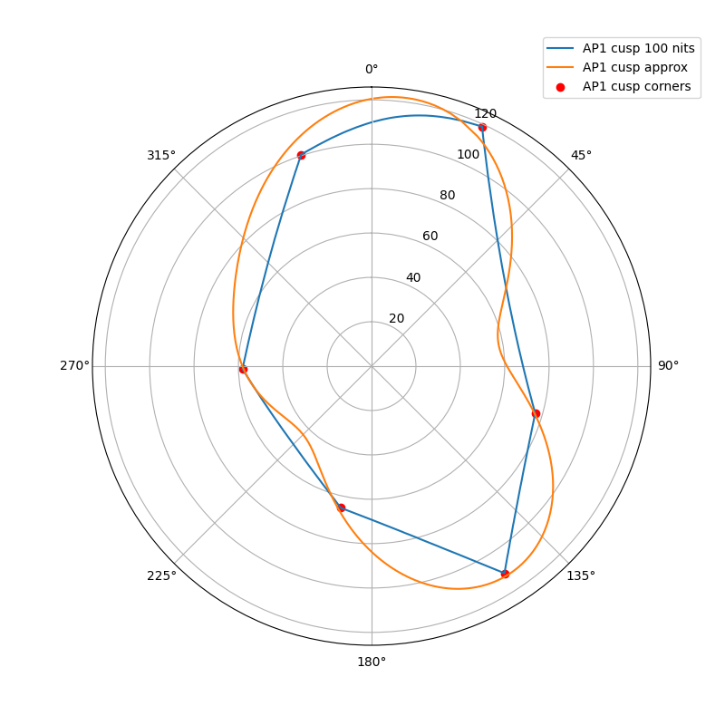
The following plots show the actual AP1 cusp (with corner dots) with the approximation for 100, 1000 and 4000 nits. What we’re looking at here is a hue circle with the cusp M values plotted.
100 nits:
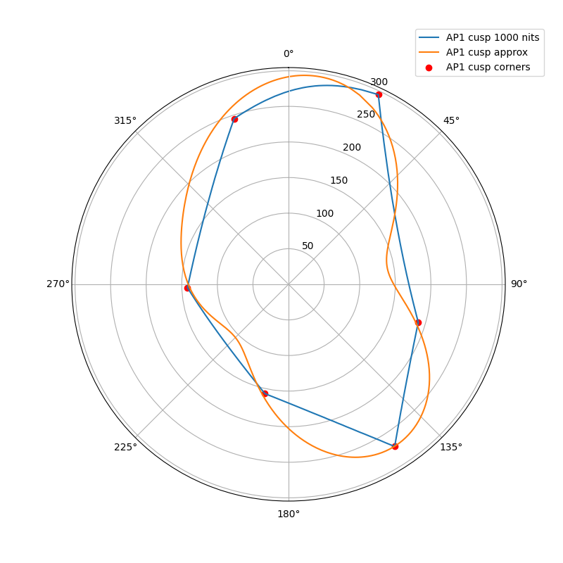
1000 nits:
4000 nits:
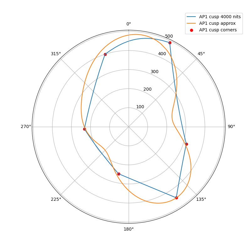
What can be seen from these plots is of course that the approximation will overshoot and undershoot the actual AP1 cusp. There’s not much that can be done about that with this kind of simple curve. It also shows that the scaling is quite consistent across different peak luminances. This means that the look and the appearance match should remain consistent across displays.
Edit: updated the plots, there was an error in the x-axis making the approximation shift to wrong location making it look worse than it actually is.
Results
The match is excellent. In fact, it’s difficult to see any differences visually. But they are there and by pixel peeping one can spot them. I’m only including few comparison images because frankly they all look identical.
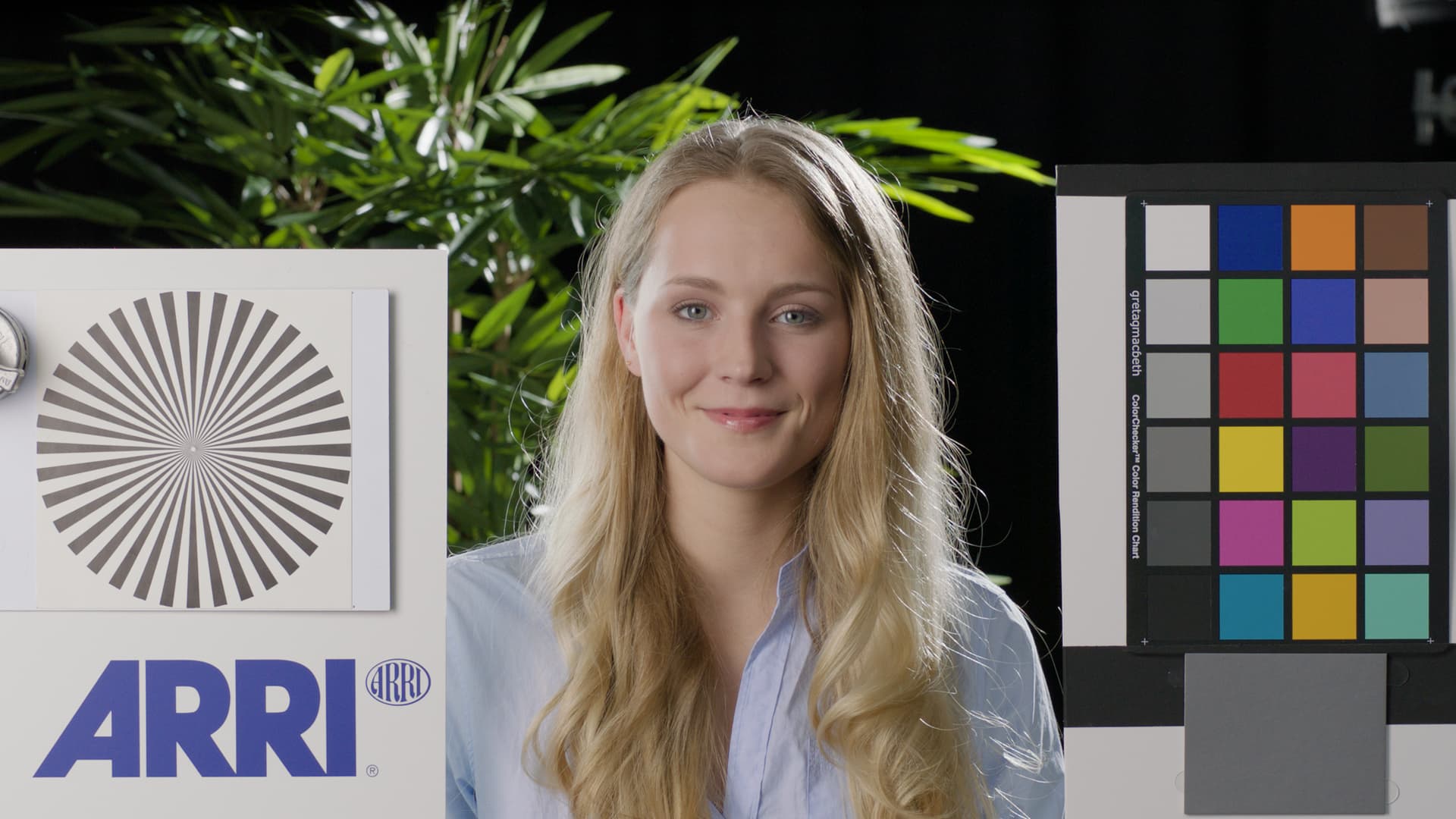
ACES2 DRT pex1 (this experiment) Rec.709:
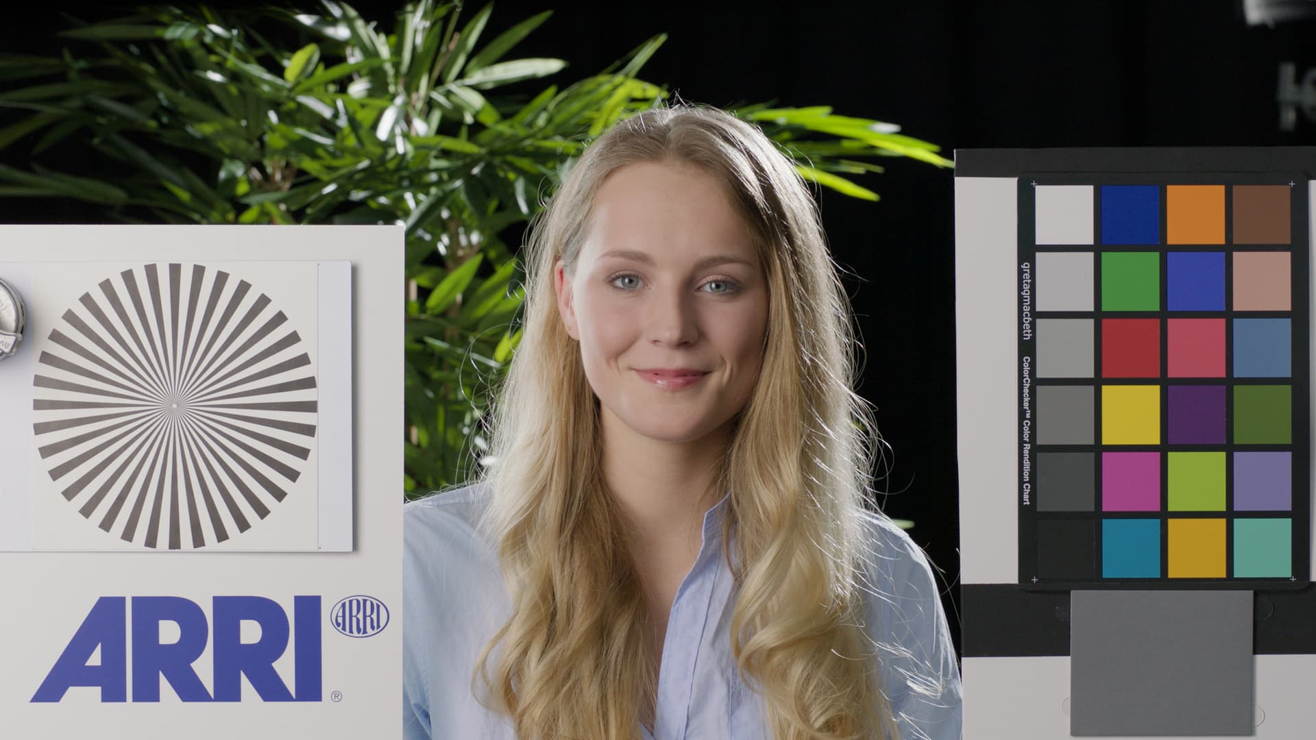
ACES2 DRT Rec.709:
Here’s the difference image of these two images, gamma up 4 to see the differences:

Average pixel difference is: ~0.000607
Max pixel difference is: ~0.014
And here’s the difference image for Rec.2100 1000 nits, gamma up 4:

Few more comparisons:
ACES2 DRT pex1 (this experiment) Rec.709:
ACES2 DRT Rec.709:
ACES2 DRT pex1 (this experiment) Rec.709:

ACES2 DRT Rec.709:
ACES2 DRT pex1 (this experiment) Rec.709:

ACES2 DRT Rec.709:
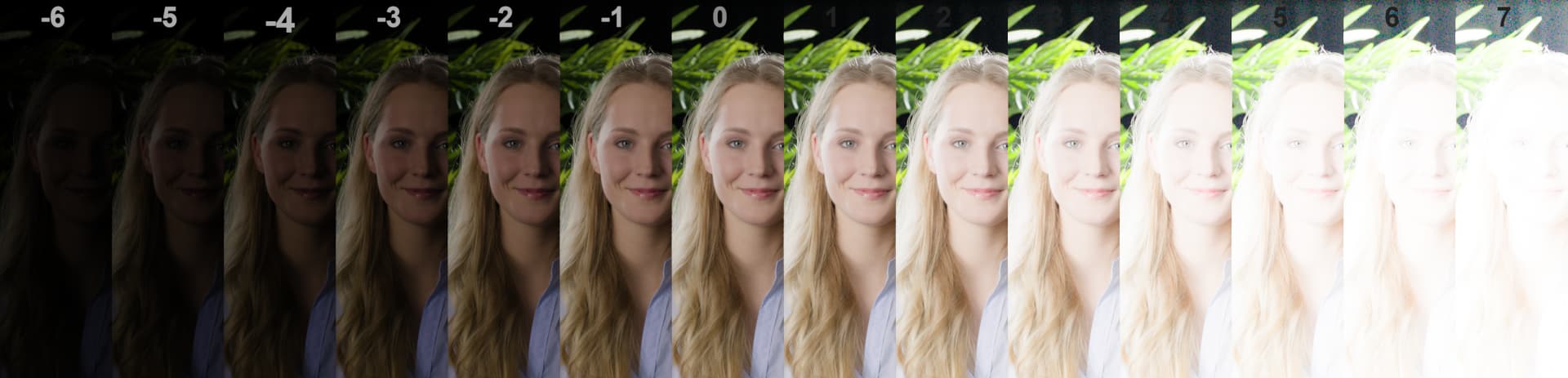
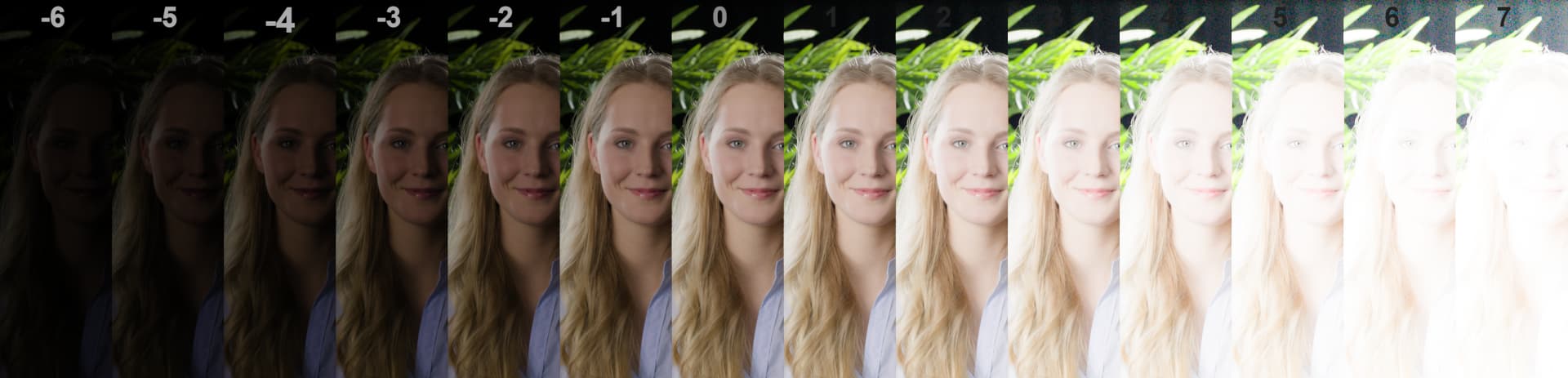
SDR/HDR appearance match
I did quick testing against 100 and 1000 nits comparing both DRT versions. Frankly it was difficult again to see the differences visually between the versions. The appearance match was as good as with ACES2 DRT.
Conclusion
If we had switched to this version at some point during development, no one would’ve noticed. The match is that close. The benefit of this approach is that there’s no more need for the AP1 cusp table and the hue dependent curve itself is not computationally heavy. Maybe this type of approach would be interesting for ACES 2.1, as it’s quite late in the day for ACES 2.0.
If you want to test this version, I’ve made it available in my prototype DRT repo. There’s both nuke node and the blink script:
ACES2_DRT_pex1.nk
ACES2_DRT_pex1.blink
The AP1 hue dependent curve is in chromaCompressNorm() function for those that are interested.