Exactly, have you tried doing the division in linear and maybe take the log of that…
Yes, the old curve essentially did that (it took log difference but same thing).
My understanding is that it is inherent in the design of the model that saturation is the ratio of M to J, so by doing that division in the model space, we are aiming to maintain saturation (at least in the way the model represents it).
And does it so?
If you make the whole image a stop brighter does this method maintain overall image appearance?
I just did an experiment, taking an SDR display-referred image, and adding gain in RGB and in Hellwig (our tweaked version) JMh (applying the same gain to J and M, and leaving h constant).
This is the result – Left is JMh. Right is RGB. Originals at the top for comparison.
(HDR display required to view this, as it is Rec.2100 PQ encoded)
It does appear that brightening an image in JMh adds colourfulness (and you can see chromaticity spread out on a CIExy scope) compared to doing it in RGB (where chromaticity remains constant). This is the opposite of what I would expect, if the model were compensating for the Hunt effect. @luke.hellwig, am I doing something wrong?
1 Like
I guess the logic is (wild guessing here):
Two stimuli with same M and h value but different J will be mapped to two different places when converted back to XYZ.
The stimulus with the higher J value is being “predicted” to elicit higher “saturation” sensation. (What ever that means)
Hence when you increase J the model adds “saturation/chroma”
This obviously is not what we want.
But again I am not familiar with this model so could be wrong.
The opposite happens actually. If saturation is roughly M / J and M is constant and only J is increased, then it will come out as less saturated. I haven’t seen Nick’s video yet, but he says he’s gaining both J and M (but J and M have different rate of change). If you increase the exposure in RGB and then go into JMh, the model will predict higher J and higher M.
Ok, it’s clicking into place for me. The model has additional background and condition dependencies in the exponent of the formula for J:
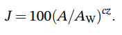 c depends on the surround conditions (‘dark’, ‘dim’, ‘average’) and z depends on the background. These are lacking from the formula for M:
![]()
So the two quantities have slightly different nonlinearities relative to light, which messes with the chromaticity when you scale both. I see two potential solutions:
- Include the cz exponent in the formula for M:
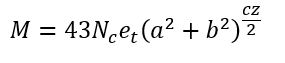
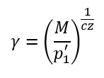
I tested this out in MATLAB and found much less chromaticity drift. Still slight, but significantly reduced. I do not think this would have adverse effects on other parts of the model. We would also have to change the formula for gamma in the inverse model:
- We could just force chromaticity to stay constant as we rescale J, instead of trying to back into that desired result with M.
6 Likes
I think that the limit parameter needs exactly the same scaling as the M channel. This way you may be able to improve the SDR/HDR matching. Without that, I got different transition points for the curve that protects purer colors.