Chroma Compression Explained

[priikone (Pekka Riikonen)]

What follows is hopefully a useful explanation of how the chroma compression works and behaves (in CAM DRT v035 as it stands). The purpose is to spread knowledge of chroma compression implementation and by visualizing its behavior hopefully inspire new ideas how to simplify and improve it.

(In some cases I will interject with extra comments about older chroma compression implementations in italic, for extra information.)

The primary input image used in the examples is an HSV sweep with 0.5 saturation:

Note that the saturation is set only to 0.5. In other words the input is not highly saturated. This is relevant because chroma compression mostly affects only the interior of the gamut.

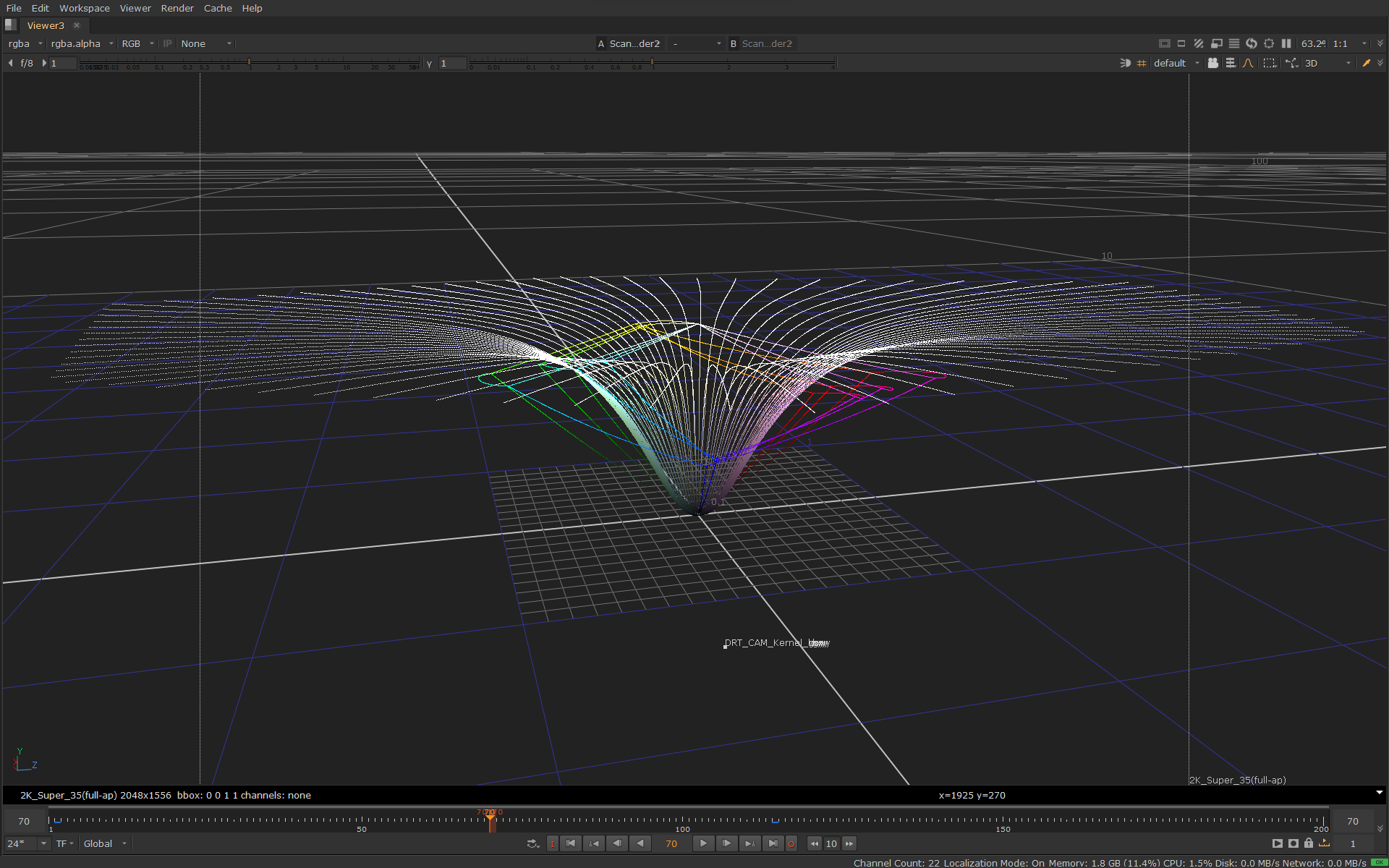
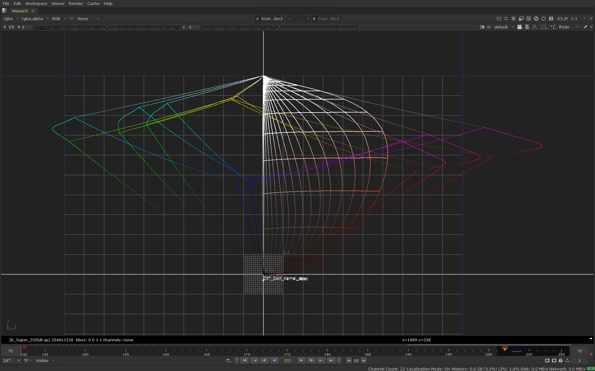
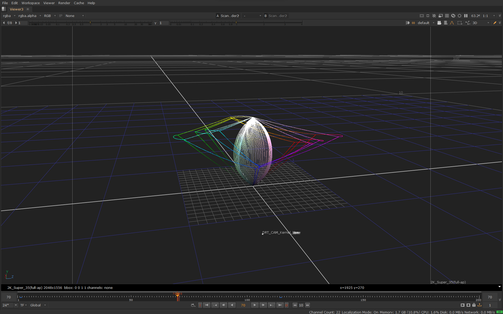
Here is the same image in 3D in JMh space going through the whole transform:

The lines in the image above also shows the JMh gamut boundaries for Rec.709, P3 and Rec.2020.

Chroma Compression

The chroma compression has three main steps:

• Scaling or normalization
• In-gamut compression or saturation roll-off or path-to-white
• Saturation boost

The purpose of these steps, with the tonescale, is to create the basic “photographic rendering”, aka. the “look” for the base transform. In practice it defines the rate-of-change for colorfulness over the brightness and colorfulness axes. I also strongly believe that better this step is and better it behaves, easier it is to color grade with the base transform.

For this post I made a modified version of CAM DRT v035 where I can toggle these three steps on and off:

The first checkbox will enable/disable the entire chroma compression. When it (“apply chroma compression”) alone is checked and others are unchecked, it applies only the scaling step. The other steps can then be added one by one.

Scaling

The purpose of this step is to bring the scene M (from JMh) values to similar range as J after tonescale has been applied to J. In simplified form, this is done by multiplying M by tonescaledJ / J:

M * (J_t/J)

In reality, though, there is an additional model on top of this for SDR/HDR appearance match. The problem of using just tonescaledJ for scaling is that the tonescales are different for each peak luminance. And, not just the peak is different (obviously), but the entire curve from shadows up, middle gray, etc. is different. This will create a visible saturation mismatch for the bulk of the image in SDR and HDR. The trick is to get the different tonescales closer to each other, except for the peak, so that the scaling ends up doing similar thing for the bulk of the image.

In v035 the full scaling algorithm to achieve this is as follows:

M*(J_t^p/J)*(1-K * c_t + 0.25)

Where the parameters are as follows:

p=0.935
K=4.4 - m_0 * 0.007
m_0 is a parameter from Daniele tonescale
c_t is a parameter from Daniele tonescale

Here’s Desmos graph to demonstrate this for different peak luminances. The parameters were derived simply by trial and error with the knowledge that for best SDR/HDR match the goal is to get the curves as close to each other as possible in shadows and at middle gray.

(if you want to see the difference between the simple scaling vs the full algorithm in SDR/HDR, CAM DRT v032 used the simplified scaling. The old chroma compression (last used in CAM DRT v031) had an engineered scaling curve and wasn’t based directly on the exact tonescale.)

In summary, the purpose of the scaling step is to scale the M to a more manageable scale, and to get the overall saturation level to match between different peak luminances, which otherwise would not.

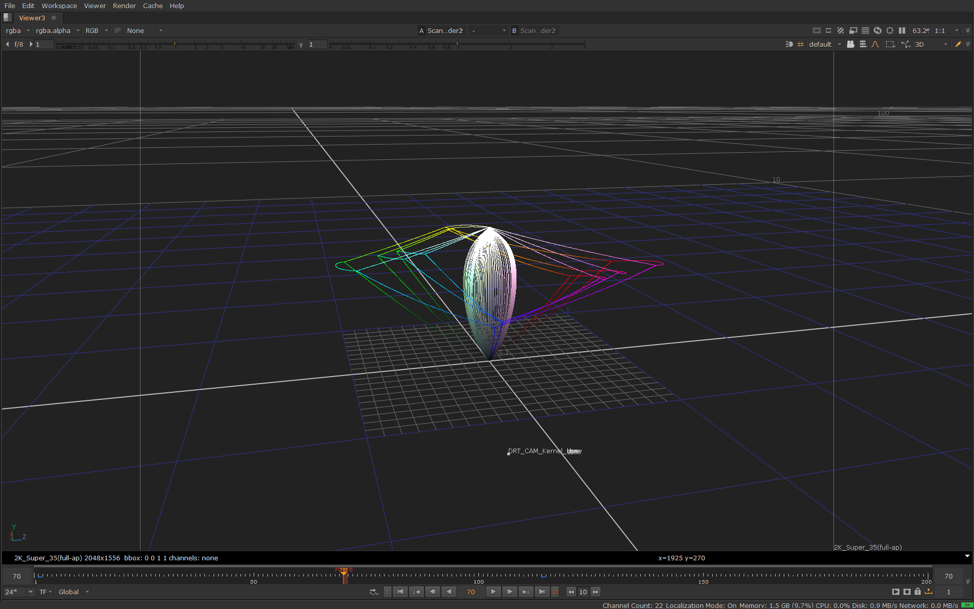
Here’s the input image in JMh space before and after the scaling step:
before scaling (shows scene M values as is (with tonescale)):

after scaling:

Note that while M has been pulled in, there is no roll-off for highlights, yet. The hue lines keep increasing colorfulness (as the model does as J goes higher) and would clip at the gamut boundary (image doesn’t show the clipping).

Here’s a slightly different input with varying chroma, with a side view of one particular hue slice, before and after scaling:

In-gamut compression

This compression step mostly creates the saturation roll-off, but it crucially takes the level of colorfulness into account as well when it changes the colorfulness. In other words, colors that are closer to achromatic are compressed different amount than colors that are far out there in the distance. The purpose of this is to both protect purer colors from being overly compressed and to create room for the bulk of the colors inside the gamut. Furthemore, it compresses brighter colors more than darker colors, creating the saturation roll-off for highlights.

Now, this step maybe deserves a post of its own to get into the nitty-gritty details. Suffice to say that the compression happens in the following steps:

• Normalize M to a compression space cusp (M / cuspM). This makes the compression also hue dependent.
• Compress the brightness/colorfulness range using this algorithm. The compression (as touched on above) is driven by the tonescaled J and the parameters can be adjusted from the DRT GUI. The compression increases for higher J but reduces for higher M.
• Denormalize M (M * cuspM)

(This algorithm was introduced in CAM DRT v032. The compression in older versions worked mostly the same way, except there was no normalization to any particular compression space and instead there was a hue dependent curve. The algorithm was different, but essentially resulting into the same thing and being driven by the tonescaled J. Before chroma compression existed the (Z)CAM DRT had a “highlight desat” mode, which was doing a global desaturation of values above middle gray. Problem with that was it was desaturating also pure colors and wasn’t hue dependent.)

Here is the result of this compression step before and after:

It’s now obvious looking at the image that highlights now have a saturation roll-off to white (or call it path-to-white). What is not so obvious from this image is how the compression affected different colorfulness levels. That’s more obvious when looking at one particular hue slice from the side with varying chroma, before and after:

Here is also a video of this compression in effect for varying chroma. Notice how the compression is significantly reduced as colorfulness increases, and vice versa:

This compression is also the reason why there is hardly any difference between full chroma compression and the simple scaling for highly saturated colors; this compression step mostly leaves those colors untouched.

Saturation boost

After the first two steps the colors in the image are looking quite dull. This is improved by boosting saturation mainly for darker colors and mid tones. The saturation boost is a simple global adjustment driven by the tonescaledJ.

M * (sat + 1.0 * (1.0 - normalizedJ_t))

An additional step to this is the desaturation of the noise floor, which is a smooth lerp to 0.01 M at 0 J. Its effect isn’t really visible unless you lift the shadows.

Here is the final result of chroma compression before and after applying the saturation boost (but before gamut mapping):

And here it is with also gamut mapping applied (ie. the full transform):

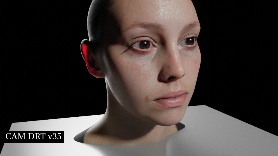
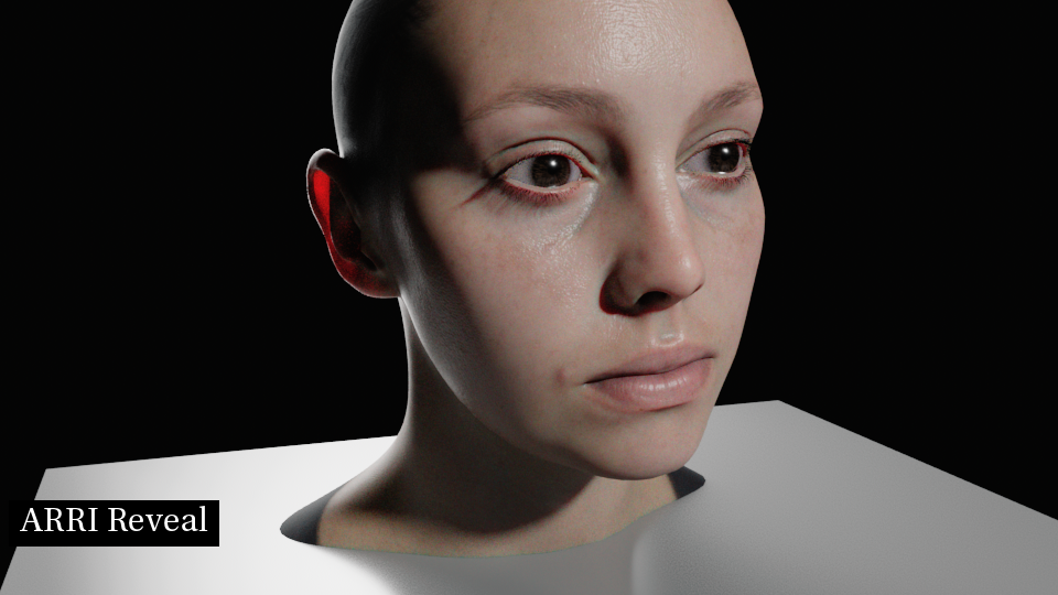
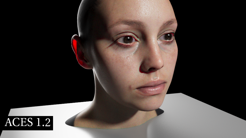
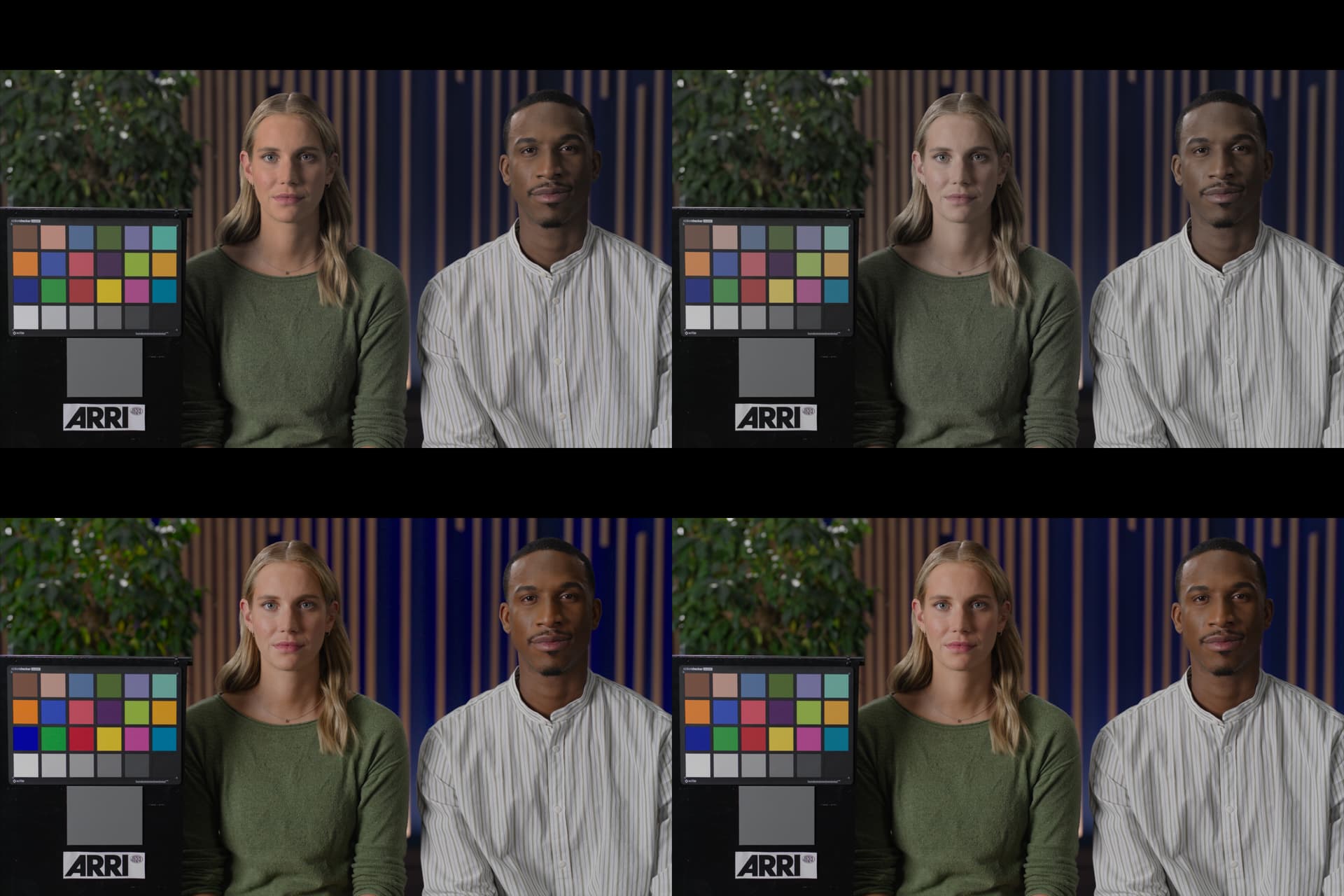
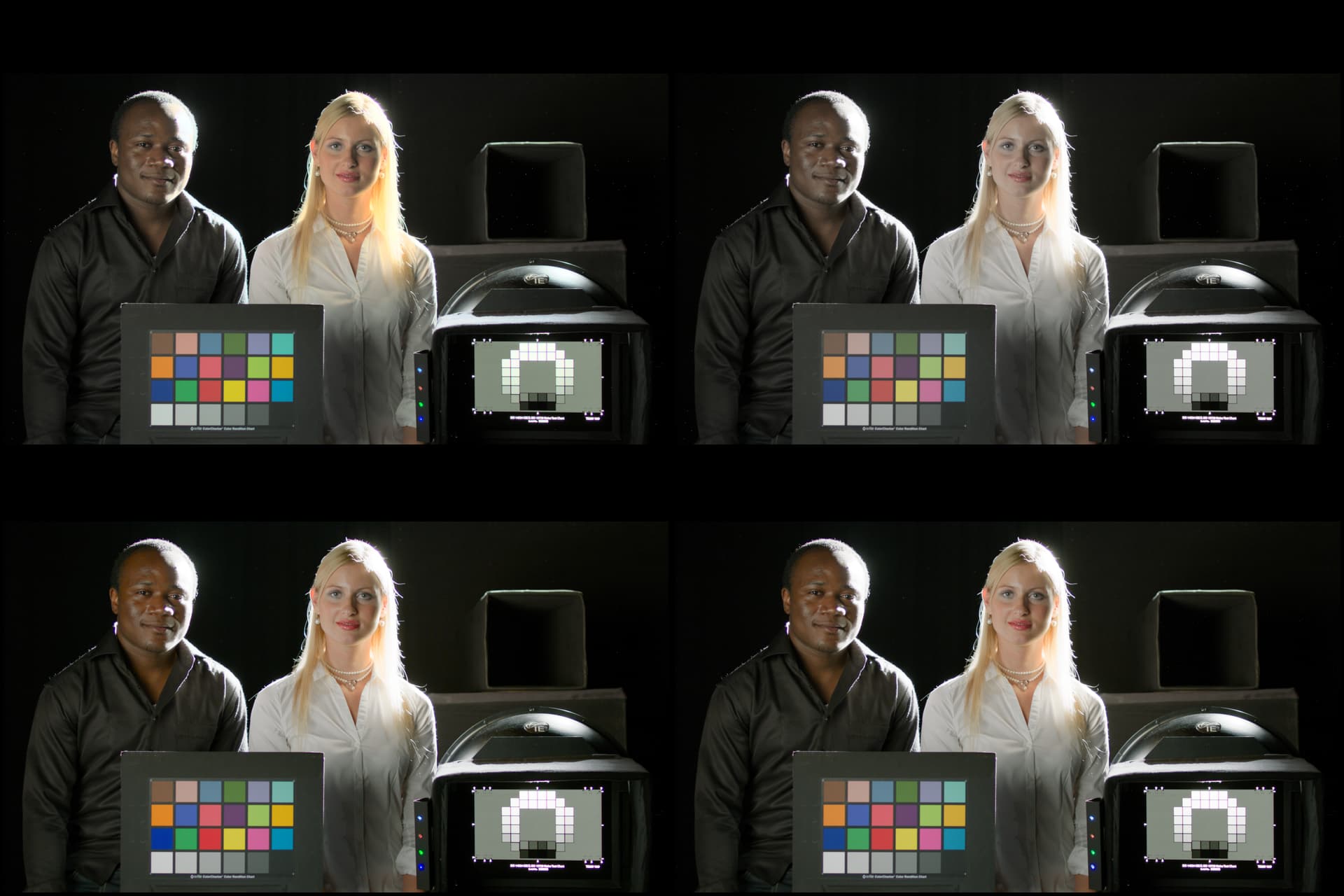
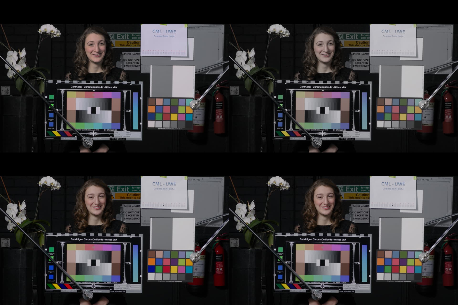
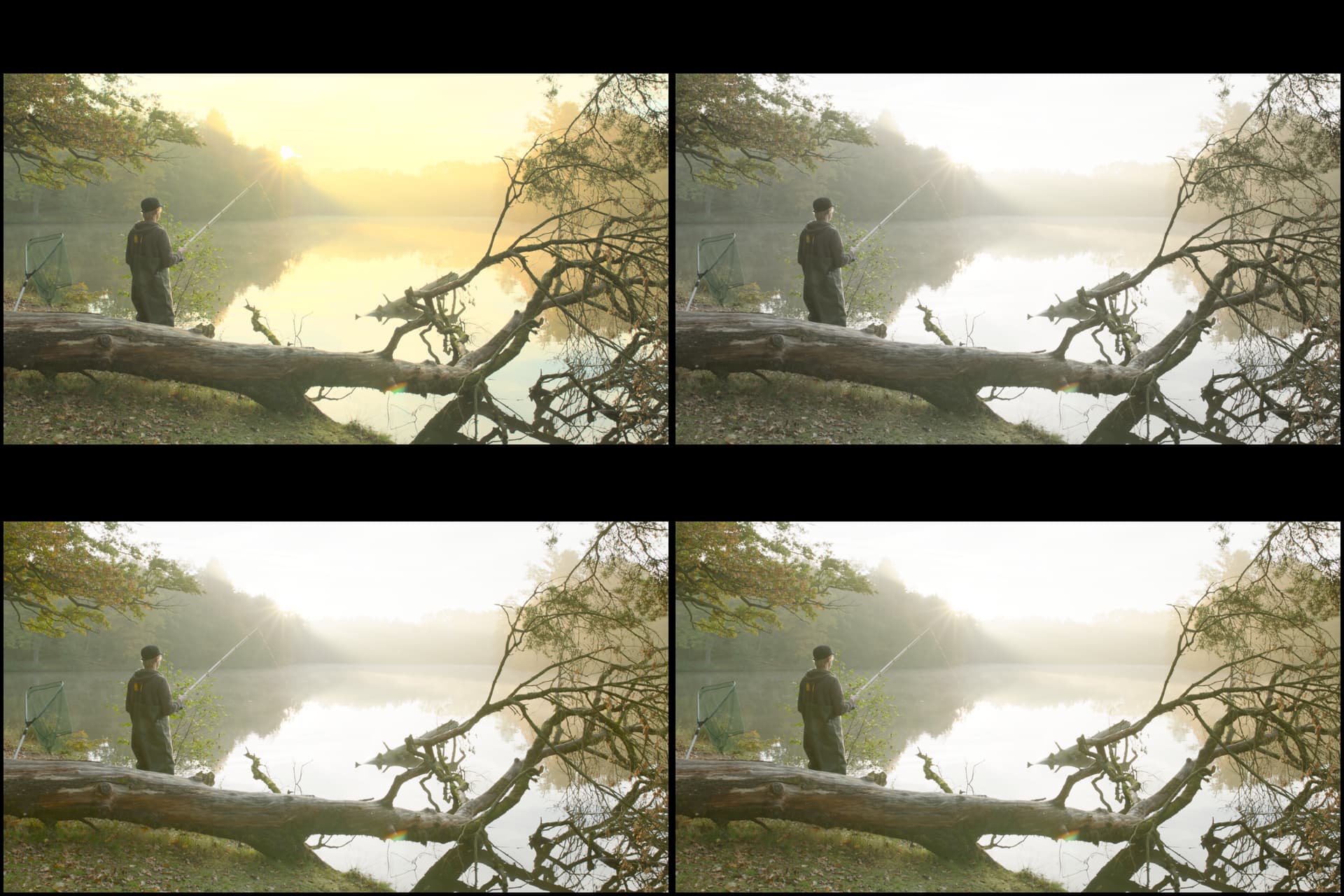
Pictures

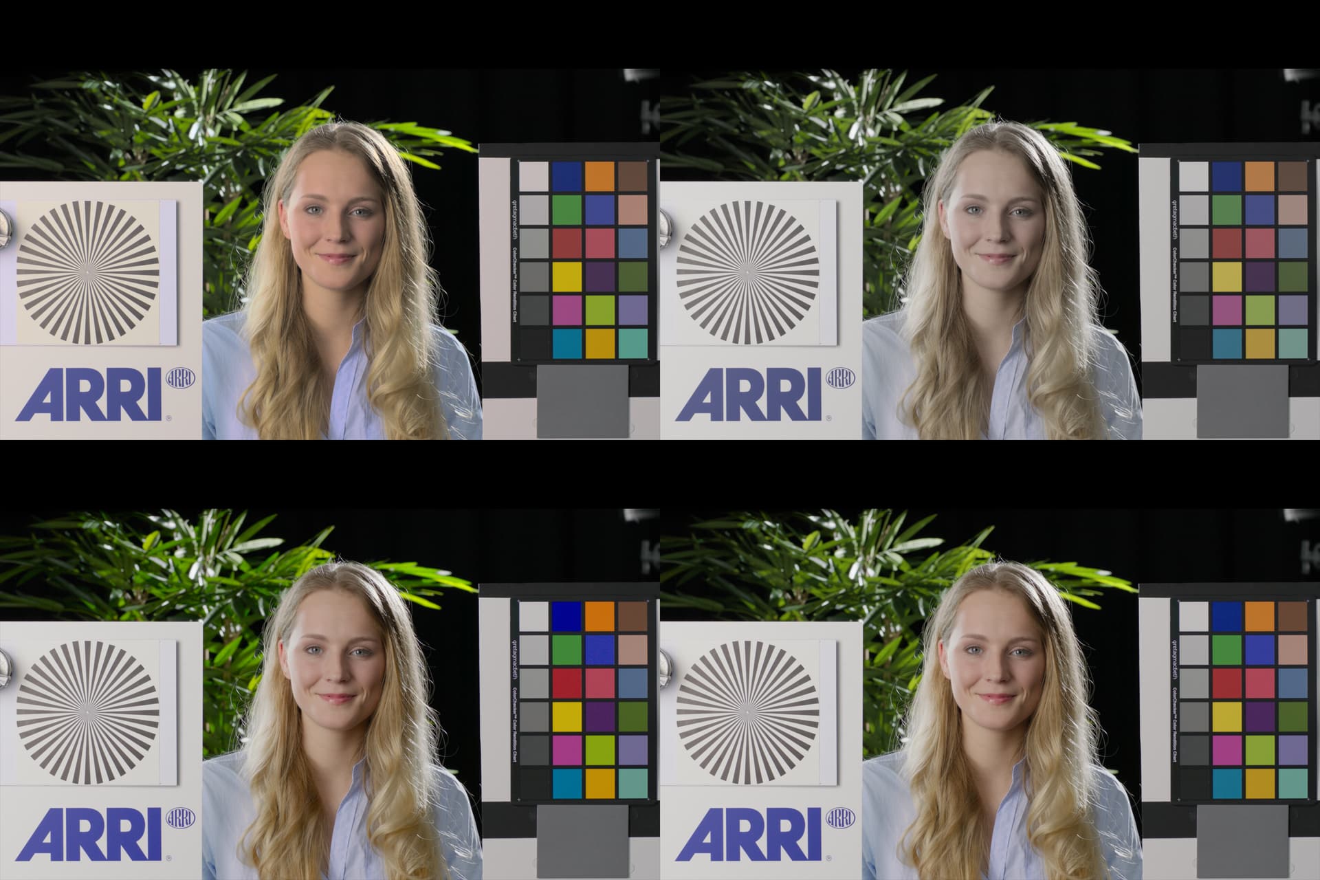
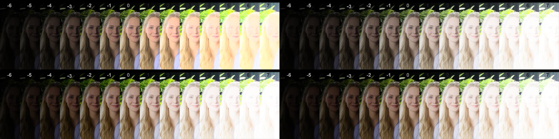
I’m not sure how useful it is to look at the intermediate steps of the chroma compression as images, but I thought I would show a few, skin tones in particular, as the colorfulness rate-of-change has a very large impact on skin tone rendering.

Sorry for not labeling the images properly.

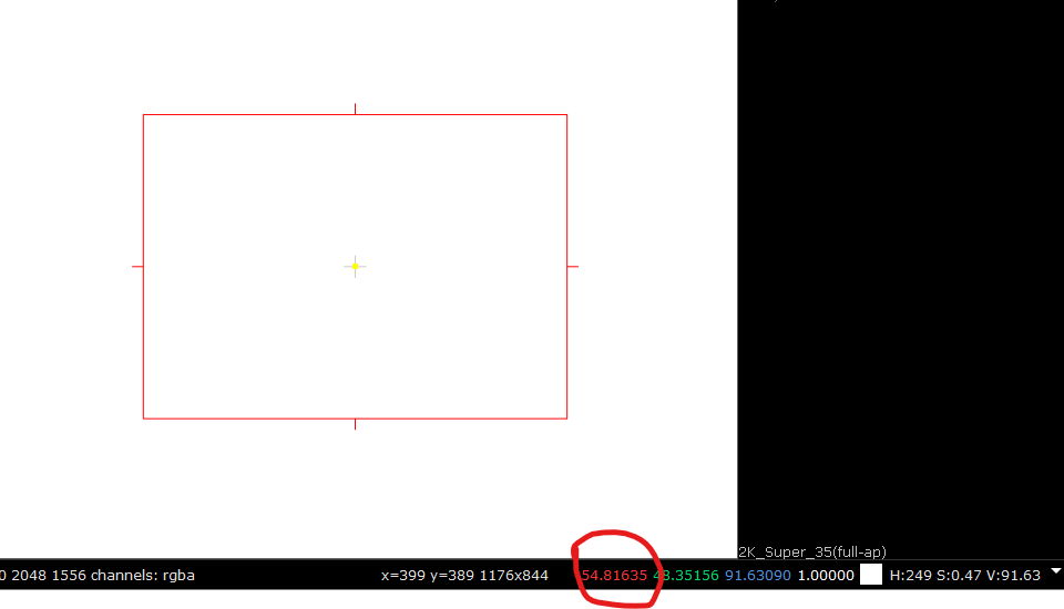
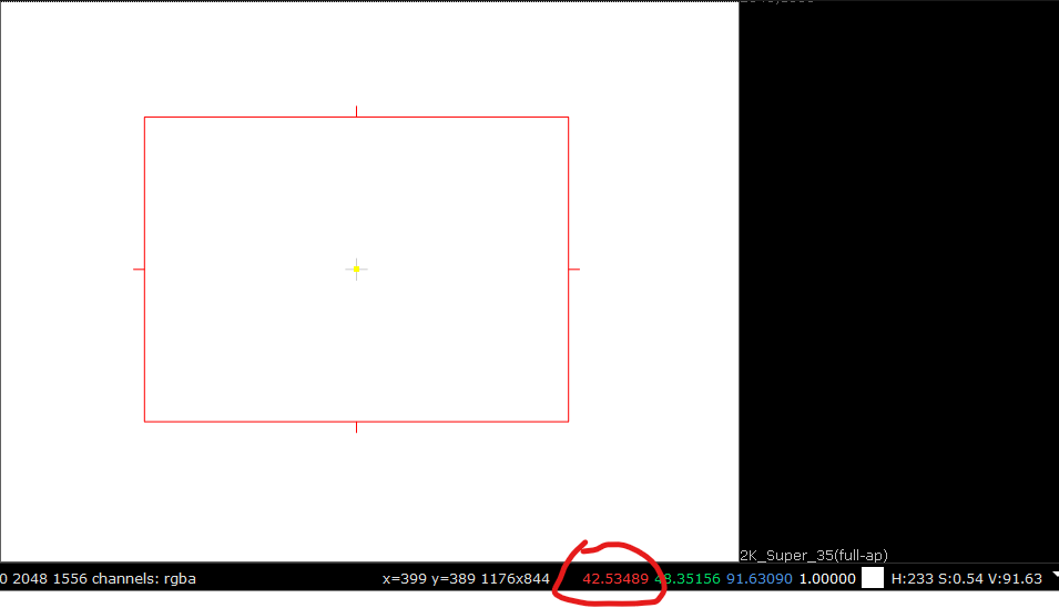
• Top left box is just the scaling step
• Top right box is with scaling + in-gamut compression step
• Bottom left box is with scaling + in-gamut compression + saturation boost
• Bottom right box is the full transform with chroma compression and gamut mapping

Known Problems

One known problem with the current implementation is the global saturation boost step which will push all colors outward, including already pure colors. The compression first went its way to protect the pure colors from over compression only then to push them even more saturated. The blue in the blue bar image, for example, will get more saturated as a result.

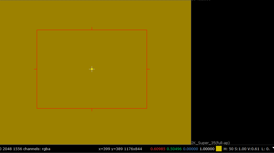
Following image is the Dominant Wavelength ramp image, and shows only those colors that were expanded beyond the original scene M values as a result of the saturation boost. Other colors not shown were under the original scene M values.

And here as an image with the yellow band being the overly boosted colors in this particular image:

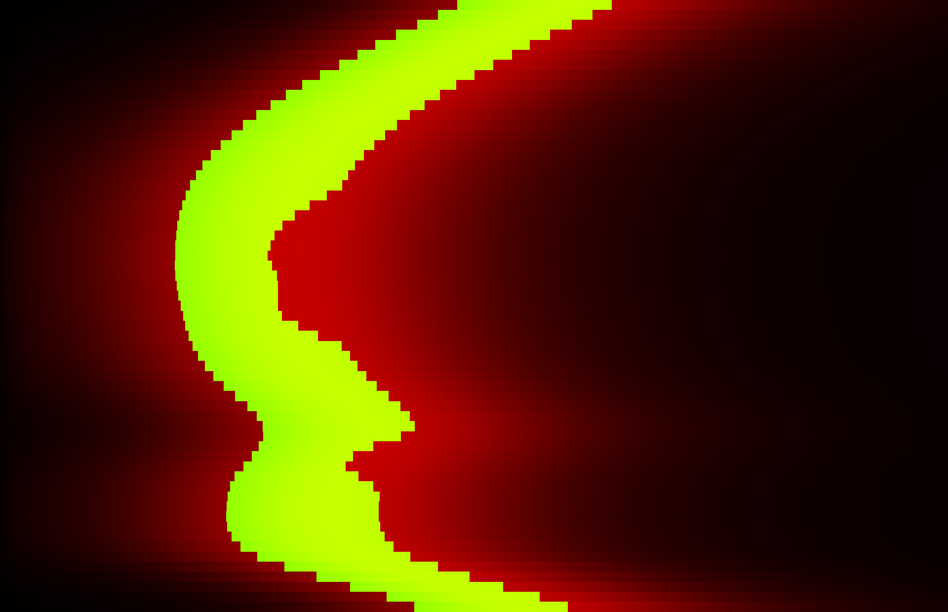
This obviously needs fixing in some way. It’s ok to boost the saturation beyond the original scene M values inside the gamut but it’s not ok to do it for these highly saturated colors that would be out of gamut any way.

I guess another known problem is the overall complexity. I must believe there is a simpler way to achieve same level of control for the compression of M and still be invertible.

[Derek]

The skin images here are really interesting to see for me. The first one (top left) looks like earlier versions of Zcam which had a sort of flat look for skin comparable to colorized photos or someone with too much caked on makeup. This really illustrates for me the importance of the chroma compression in getting to the final image.

Inspired by this I wanted to revisit how CAM DRT v35 looked on CG skin. I was really happy with the results.

This is Digital Emily2, all images output in BT1886. First image is CAM DRT v35. I really love how the translucent nature of skin is coming through here.

Compare that to ARRI Reveal which has a similar “translucent” appearance, with the main difference I observe being that ARRI is less saturated. I personally prefer the bright punchy colors of the CAM DRT.

Finally we have ACES 1.2 with all the familiar issues of how skin looks there.

Having followed the development of the ODT through its many iterations, it’s really exciting to see this state of things. Looks amazing!

[alexander-behm]

Thank you for describing the chroma compression algorithm!

Are you aware of this paper? https://www.cl.cam.ac.uk/~rkm38/pdfs/mantiuk09cctm.pdf

I think they are discussing a solution for the same problem.

EDIT: Here is another paper that builds on the same formulas: https://user.ceng.metu.edu.tr/~akyuz/files/saturation.pdf

[daniele (Daniele Siragusano)]

At that time of

@alexander-behm

Are you aware of this paper?

At the time those paper try to achieve a "more preferred " rendering
on an SDR display. Also they do not examine how the same appearance can be achieved on different displays I guess.

[priikone (Pekka Riikonen)]

There is now v039 in my fork of Alex’s repo, which has the chroma compression split into separate toggleable steps.

[priikone (Pekka Riikonen)]

While developing a new variant of chroma compression that wouldn’t need the saturation boost step, I’m coming to a conclusion that saturation boost is needed in order to be able to create the appearance match between different displays.

The reason is that normal range of colors actually end up less saturated as a result of the differences in the tonescale, namely how much the middle gray is lifted. Following video shows the effect the tonescale has to J and M. This shows the tonescale step alone; there is no chroma compression, no scaling, no roll-off, or gamut mapping happening. The video shows me switching between 100 nits, 1000 nits and 4000 nits tonescales and back. The widest one (most saturated one) is the 100 nits and the narrowest (least saturated one) is the 4000 nits. What the video shows is how higher nits tonescale will result into desaturation in the region shown. Only way to recover the lost saturation is to boost it (reducing chroma compression wouldn’t be enough to compensate. Even disabling the chroma compression wouldn’t be enough for the 4000 nits curve).

In testing I have found that by lowering how much middle gray is lifted would be one way to address this. Another way is to do the saturation boost. And yet another would be to lower the saturation of the 100 nits rendering to create better match.

What the video of course doesn’t show is that how much higher up 1000 and 4000 nits curves extend compared to the 100 nits. But in this case the region of interest is the normal range and middle gray region, and to show how the tonescales affect it.

[priikone (Pekka Riikonen)]

Here’s another take on a video showing this. This time it’s showing one hue slice with a horizontal line included so that it’s easier to see where the points along that line end up as J is compressed less with higher nits tonescales. I left the mouse cursor on the spot on the 100 nits curve I was following. I’m switching between 100, 250, 500, 1000 and 4000 nits tonescales, and back.

The M of course doesn’t change, only J changes, and the ratio of those two. Same as with previous video, this shows only the tonescale step. There’s no chroma compression or gamut mapping applied.

The chroma compression creates the appearance match of course, but the problem is that higher nits rendering without chroma compression applied may look less saturated than fully chroma compressed 100 nits rendering for certain colors. So increasing saturation would then be only way in that case to match them, or to lower the saturation of the 100 nits rendering. The tonescaledJ / J ratio can’t recover it (unless we let the ratio to go >1.0, which then would increase the saturation).

Not sure how relevant it is but it’s also clear looking at post-transform display RGB saturation values that they’re getting lower as the tonescale peak is increased (for certain colors). And, that by increasing the saturation, I feel the appearance match gets better.

[nick (Nick Shaw)]

@priikone

The chroma compression creates the appearance match of course, but the problem is that higher nits rendering without chroma compression applied may look less saturated than fully chroma compressed 100 nits rendering for certain colors. So increasing saturation would then be only way in that case to match them, or to lower the saturation of the 100 nits rendering. The tonescaledJ / J ratio can’t recover it (unless we let the ratio to go >1.0, which then would increase the saturation).

I don’t completely follow this. Since M is multiplied by \frac{J_{toneScaled}}{J} for both the 100 nit and 1000 nit versions, surely you don’t necessarily need the 1000 nit M multiplier to be >1 for a match. You just need it to be greater than the 100 nit M multiplier, as we are talking about matching saturation (\frac{M}{J}) between the two.

@priikone, you talk about us “increasing J” at higher peaks. But surely we are not increasing it. We are decreasing it less than we do for SDR, which is not the same.

Ignoring the fact that the tone-scale is a curve, for a given input value it is multiplying J by a fraction, which is different for SDR and HDR. Let’s call those fractions k_{SDR} and k_{HDR}.

J_{toneScaledSDR} = k_{SDR} \times J

J_{toneScaledHDR} = k_{HDR} \times J

In the first chroma compression step we multiply M by \frac{J_{toneScaled}}{J}, which is the same as each of the two k values.

So the saturations are:

Sat_{SDR} = \frac{M_{SDR}}{J_{toneScaledSDR}}=\frac{k_{SDR}\times M}{k_{SDR}\times J}=\frac{M}{J}

and

Sat_{HDR} = \frac{M_{HDR}}{J_{toneScaledHDR}}=\frac{k_{HDR}\times M}{k_{HDR}\times J}=\frac{M}{J}

So the saturation of the original, the SDR and the HDR are all \frac{M}{J}. So it appears, unless I have misunderstood, that with the simple chroma compression we do preserve saturation. So does this mean that preserving \frac{M}{J} in the model does not in fact produce a match for different J values? Or is it just that the additional in-gamut compression needed to produce a “pleasing image” changes things so saturation is no longer preserved. If the latter is the case, it might suggest that we need to apply the necessary modification before tone-scaling and a simple chroma compression (an LMT in JMh, if you like) in order to achieve a match at different display peaks.

[priikone (Pekka Riikonen)]

@nick

surely you don’t necessarily need the 1000 nit M multiplier to be >1 for a match. You just need it to be greater than the 100 nit M multiplier

First, the 1000 nit J_t/J is going >1.0. If we don’t do anything to that, it will increase saturation on its own. But we want to be able to control it.

Second, yes, I am saying that given how saturated the 100 nit rendering is that if you multiplied the 1000 nit M by 1.0 (ie. didn’t compress it at all), there is not going to be appearance match and the image looks less saturated than 100 nits. 10000 nit rendering for those colors is the least saturated.

@nick

We are decreasing it less than we do for SDR, which is not the same.

It’s true we are decreasing J less with 1000 nits than 100 nits. But, we are increasing it with ~2000 nits and above. 10000 nits is way above the original J scene value!

Here’s a color patch, first in RGB, second scene JMh, third 100 nits tonescale JMh, fourth 1000 nits tonescale JMh, and fifth for 10000 nits JMh. Notice the increase in J (red channel) between 100 and 1000 nits. Notice also how the M (green channel) does not change. And notice the 10000 nits J is above the scene J.

RGB:

scene JMh:

100 nits JMh:

1000 nits JMh:

10000 nits JMh:

So, the resulting saturation (M/J) decreases. And the 100 nits rendering being the reference we match against, the difference is visible.

Now, I was hoping that it would be enough to just scale the J_t/J so that when it’s close to 1.0 (and above the 100 nit multiplier) it would produce enough saturation for there to be a match (as you said in your post). What I found is that’s not the case and that’s what the first post on this issue was about. It’s close enough for 1000 nits that it can be argued about, but will go way off with higher nits (plus rest of the chroma compression will bring additional compression that also needs to be kept in mind for the appearance match). My tests were with full chroma compression disabled; things get even less saturated with it enabled, naturally, but it’s not the cause.

Hopefully my explanation makes this a little bit clearer.

[nick (Nick Shaw)]

But in my equations above, it should not matter if k_{HDR} (or k_{SDR}, for that matter) is <1 or >1. It cancels out with only \frac{J_t}{J} scaling. If the tone curve takes display J above scene J for a particular value, then surely M should be increased – the cone of the spectral locus keeps getting wider as J increases. It would seem that doing additional processing to keep the M scale below 1 is a potential cause of the desaturation. Anything which changes the \frac{M}{J} ratio is literally changing saturation, because \frac{M}{J} is the definition of saturation in this model.

The M scaling going above one is not a saturation boost. It is a colourfulness boost. But surely that is appropriate to maintain saturation as J increases.

[priikone (Pekka Riikonen)]

That is my argument as well, and was the conclusion I came to in that first post. However, I don’t believe the model will give us the match we want just by using the pure ratio. We want to be able to control it ourselves for the best match, and to avoid having to make the in-gamut compression peak dependent. In testing I have concluded that the pure ratio would give overly saturated image in HDR and would require the in-gamut compression to do something very different for each tonescale.

There is going to have to be a point in the transform where the appearance match is created, given the purpose designed mismatching tonescales. I’ve chosen to do that in the scaling step because I believe that’s the easiest place to do it. The only other place to do it would be the in-gamut compression step, but I believe it would be more difficult to do it with that, with the current technique.

We could make our lives a little bit easier if the middle gray wasn’t lifted quite as much between 100 and 1000 nits (as I’ve brought up a few times), or by reducing the 100 nits rendering saturation a smitch. Then the 1000+ higher nits can be dealt with the “hunt compensation” or “colorfulness boost”.

[daniele (Daniele Siragusano)]

I hardly can follow you guys into that rabbid hole…

But:

Surely you want to (If anything) decrease chroma If you move luminance up to compensate for the Hunt effect. TBH I don’t think this is a major parameter for a match between SDR and HDR from my experience, so I guess you are chasing something else.

Then when you say “this gives an appearance match between SDR and HDR” how exactly do you judge this.
How long do you let yourself adapt to the new viewing condition, (see Contrast Gain Control)?

Contrast Gain Control

Then when you say you want to tweak on top what “the model” provides, why are you using the model in the first place then?

Also if you are not happy with the pre and post tonemap ratios to drive any other scale, maybe you shouldn’t .
Are you taking the original linear light ratios or some other form like PQ ratios?

[nick (Nick Shaw)]

@daniele

Are you taking the original linear light ratios or some other form like PQ ratios?

It is the ratio of Hellwig J before and after tone mapping. We (as a first step) multiply M by that ratio to scale it down by the same amount the tonemap has scaled J by, in order to maintain saturation (which is defined in the model as M / J) through the tonemapping.

(this was originally suggested by @luke.hellwig as something that should be done if using his model)

[daniele (Daniele Siragusano)]

So you taking the values before and after a linear light tonemapping function, then convert it to some JND based encoding (PQ ish I guess) and then take the ratios.
What do those ratio even mean?

[priikone (Pekka Riikonen)]

@daniele

Surely you want to (If anything) decrease chroma If you move luminance up to compensate for the Hunt effect.

We’re not doing this, as far as I understand it. I would not get hung up on Hunt or anything like that when it comes to scaling the M (colorfulness). I consider doing that, and creating the appearance match, a purely technical step.

The first post of this thread tries to explain how the current compression works and behaves, including how the tonescale changing J over J (J_t/J) is currently used to do the scaling of M, but it also references older versions of the compression that have used entirely different method, not based on pre/post tonescaled ratios. There has been many many different versions, including using the derivative of the tonescale, but the current one works and is the simplest one, even with the extra tweaks needed to get the compression to a similar starting point for different displays (different tonescales) that can create a reasonable appearance match. It doesn’t matter much to me how the scaling of M is done, as long as it is simple enough and affords the necessary control I believe is needed to create the appearance match, and to get the behavior we currently have. I absolutely do not believe there is “one correct” curve to do it.

The discussion me and Nick are having is about trying to make a simpler version of what’s explained in the first post of this thread that would not need the extra colorfulness/saturation boost step. I’ve got that working quite well, but not necessarily any simpler… The scaling is the part that sets the overall base colorfulness level with each tonescale for the match.

If you have an alternative idea, tonescale based or not, that we could use, I would be very happy to hear about it.

@daniele

How long do you let yourself adapt to the new viewing condition, (see Contrast Gain Control)?

Thanks for that link, I will keep that in mind. Personally I spend a long time comparing the images, especially in situation like this where I’m changing the appearance match. I favor doing A/B comparison with Rec.709 sim and Rec.2100, but I do side by side comparisons on same screen as well. My personal benchmark for the quality and performance of the appearance match is ARRI Reveal. Can’t be a bad match if we can get close to performance like that…

From earlier discussion:

@daniele

As long as you leave hue alone, you are fine. Then you could scale a,b directly using M as a modulator.
But if you start to tinker with hue-specific tweaks I think you are off the rails.

How would you approach using M as the modulator and do it in a way that’s invertible? We are using M as the modulator and the current approach is invertible, but I am on the look out for any other way or technique that could be used to achieve it. There’s plenty of ways I can think of that aren’t invertible (we obviously don’t have the original M available in the inverse). Any tips and help would be highly appreciated.

[daniele (Daniele Siragusano)]

I am confused:

In your original Post you write:

@priikone

The purpose of these steps, with the tonescale, is to create the basic “photographic rendering”, aka. the “look” for the base transform.

Now you write:

@priikone

I would not get hung up on Hunt or anything like that when it comes to scaling the M (colorfulness). I consider doing that, and creating the appearance match, a purely technical step.

If this ist a “purley technical step”, what is your cost function? Surely there needs to be an objectiv metric.

A Look operation should not need any tweak for different viewing conditions. Otherwise the DRT is not functioning correctly.
If you are working on the appearance match of the DRT, you need to modify the model and not hand tinker with the parameter of the model.

The more I think about it J_t/J is probably a bad driver. Probably this is why your M modulation is so sensitive to shadows/greys. If you do some sort of log of the linear ratios you might get something that behaves better.

[priikone (Pekka Riikonen)]

@daniele

If this ist a “purley technical step”, what is your cost function?

The look is created in the second step. That is the “base transform look”, and yes it does not need any tweaks to viewing conditions or anything else like that. Very much subjective step.

The first step is the scaling step which also creates the appearance match. That is what Nick and I were talking about. The first step is the technical step, or one could call it even a normalization step, and that then allows the second step to not need any tweaks, even though the output is for different displays.

I could not figure out how to do both in one step (at least not in invertible way, the very first version did that, but was very naive and not invertible)).

@daniele

The more I think about it J_t/JJt/JJ_t/J is probably a bad driver. Probably this is why your M modulation is so sensitive to shadows/greys.

What do you mean by sensitive? Do you mean it compresses them clearly different amount or that it has to, or something else?

@daniele

If you do some sort of log of the linear ratios you might get something that behaves better.

I believe the previous chroma compression version was actually doing something like that. It wasn’t the linear ratios of the tonescale itself, but another similar curve. It’s the one I linked in the first post. That thing is too complicated but I could probably come up something much simpler now, but still more complicated than the current approach. Simplicity was the reason why I switched…

[daniele (Daniele Siragusano)]

@priikone

The first step is the scaling step which also creates the appearance match. That is what Nick and I were talking about. The first step is the technical step, or one could call it even a normalization step, and that then allows the second step to not need any tweaks, even though the output is for different displays.

Is this the right order?
Intuitively I would assume you do a “look” transform which then is translated to various viewing conditions. The same order would be present with any custom LMT prior to the DRT…

@priikone

What do you mean by sensitive?

A division in log is very different that a division in linear light.

[priikone (Pekka Riikonen)]

@daniele

Is this the right order?
Intuitively I would assume you do a “look” transform which then is translated to various viewing conditions

It is a valid question, but I can probably envision a more complicated solution for it. In the end they should end up in a very similar place. I have not tried to do this…

I also want to address this because I think it’s important:

@daniele

If you are working on the appearance match of the DRT, you need to modify the model and not hand tinker with the parameter of the model.

This is a path I have chosen not go down. I wouldn’t know where to start. I’ve chosen to work with the CAM rather than develop an alternative CAM. I’ll leave that to someone else. I think both approaches are valid.

[priikone (Pekka Riikonen)]

@daniele

@priikone

What do you mean by sensitive?

A division in log is very different that a division in linear light.

The J_t/J is not in linear. We’re doing it in the non-linear model space.