Hi all,
I’ve been following this thread with great interest. I’ve plotted a selection of compression functions here: https://www.desmos.com/calculator/9rfpgk1iae
All exhibit C1 and C2 continuity and have straightforward inverses. The “Power(2)” option is a middle-ground between tanh and arctan. The “Power( p )” option is tweak-able and works well with p values in the range [1.5, 3].
I think it would be interesting to see Thomas’ Float16 domain test applied to these functions. I’ve run out of time today, but I might get round to it later in the week.
I added the “power” compression function with default parameter of p=2:
def power_compression_function(x, a=0.8, b=1 - 0.8, p=2.0):
    x = colour.utilities.as_float_array(x)

    return np.where(x > a, a + (((x - a) / b) / np.power(1 + np.power((x - a) / b, p), 1.0/p)) * b, x)
which gave these results:
[ Threshold 0.0 ]
tanh 6.58594
atan 7376.0
simple 23168.0
power 161.25


[ Threshold 0.1 ]
tanh 6.02734
atan 6636.0
simple 14744.0
power 115.312


[ Threshold 0.2 ]
tanh 5.46875
atan 5900.0
simple 13104.0
power 102.625


[ Threshold 0.3 ]
tanh 4.91016
atan 3650.0
simple 8108.0
power 89.875


[ Threshold 0.4 ]
tanh 4.35156
atan 3130.0
simple 6952.0
power 61.3438


[ Threshold 0.5 ]
tanh 3.61914
atan 1844.0
simple 5792.0
power 51.2812


[ Threshold 0.6 ]
tanh 3.0957
atan 1476.0
simple 3278.0
power 41.25


[ Threshold 0.7 ]
tanh 2.57227
atan 783.0
simple 1738.0
power 24.8906


[ Threshold 0.8 ]
tanh 1.97852
atan 369.5
simple 820.0
power 13.6016


[ Threshold 0.9 ]
tanh 1.48926
atan 93.0625
simple 205.625
power 5.98047


[ Threshold 1.0 ]
tanh 1
atan 1
simple 1
power 1
The test identifies the first point at which the difference between adjacent compressed values is “very small” (sufficiently small that when converted to float16 it rounds to zero). I suppose this test is analogous to finding the point at which the gradient is <= a fixed threshold, but not exactly the same due to the distribution of floating point values.
I’m taking it to be a relative metric of how ‘aggressive’ each function is; in order of mild->aggressive we get:
Wow! Thank you so much for these. This is extremely helpful.
I would be very curious to see if any of these functions can be solved such that a parameter could specify the x value that intersects 1.0.
To expand on that:
At least for the DCC implementations of this idea, the distance limit parameters specify the distance beyond the gamut boundary to compress to the gamut boundary.
To do this, the compression functions need to be solved for the y=1 intersection. A value of L needs to be calculated for the compression function that results in the curve intersecting y=1 at x=L.
Here’s a plot of the Reinhard compression function to demonstrate the idea. Reinhard Compression Function | Desmos
In the first plot, L specifies the asymptotic limit. In the second, L specifies the y=1 intersection.
All of the other compression functions that we’ve come up with so far are not directly solvable in this way (or to do so is beyond my limited math ability).
To solve these other functions currently I’m implementing a bisection solver to calculate the limit value. It adds complexity to the code and there is nothing I would like more than to remove it.
For the record, here are the other compression functions that we’ve come up with so far. Each plot includes the inverse function, the y=1 x value, and the 2nd derivative. These are sorted by aggressiveness of the curve. log reinhard exp arctan tanh
Since your math skills are obviously several steps beyond min, I would be very curious to hear your thoughts on whether it is possible to solve any other of these compression functions for the y=1 intersection in the same way as the Reinhard function.
Also I’m very interested in the “Power( p )” function, as it might allow us add “slope” as an additional parameter.
There should not be real surprise that by fiddling with the parametrisation the curves will eventually produce an output relatively similar for a given domain, they all share the sigmoid trait.
The good function is the one that preserves purity at the highest possible limit, i.e. not a small domain, while being free of defects.
I’m tempted to say that if anything, your images show that tanh is almost ideal over a small distance
C2 continuity will guarantee identical curvature at the graft point which prevents steep slope from the function you are appending. B-Splines are C2 continuous so as mentioned somewhere above we could also look into that but I don’t feel like it is warranted and it would certainly complexify the implementation.
Something to keep in mind is that the numbers I gave above (along those extended by @JamesEggleton) are for HalfFloat computations thus it is extreme case scenario as high quality image processing will happen with at least single-precision 32-bit representation. There are of course real-time applications that use HalfFloat happily for processing but in the context of this group this is no-concern.
I will re-run the notebook with Float32, hopefully the Colab VM does not run out of ram
Although internal processing should be at least Float32, we can’t ignore the fact that people will (unofficially) store ACEScg data in half-float EXRs. If that data has been through the gamut mapper, then it is half-float quantisation which matters if the gamut mapper is to be subsequently inverted.
Yes agreed, I was just highlighting that this is an extreme case scenario.
Practically speaking anyway, none of the function will ever come close to 65504, there is point where it does not matter though, I don’t know where is that threshold unfortunately. As an engineer/developer I’m certainly mostly concerned about preserving as much of the data possible however as an artist (I have the great pleasure of wearing both caps) I don’t really care that much about how far the values are coming from, what is important to me is where they do land upon mapping, i.e. maximum purity.
Colab died btw, will have to pull the notebook locally!
Here is what I understand from what you are saying:
An ideal compression function will preserve the most color purity with the smallest threshold value. That is, if two compression functions are compared with the same threshold value and limit, the one that preserves the most purity would win.
And unfortunately to preserve the most color purity, the slope has to be very “aggressive”. The more aggressive the curve, the more problems there are going to be with invertibility with half float precision. So a compromise between the two must be reached.
Yes exactly! It will have to be a compromise. I’m not sure exactly which one because I’m myself dancing from one foot to another as you saw in my engineer vs artist reply just above
It turned out to be straightforward to solve the “Power( p )” function for the y=1 intersection.
I’ve implemented the functionality here: https://www.desmos.com/calculator/zifabox6lr
You can tweak the threshold (t), the point that the graph must pass through (x0,y0), and the power ( p ).
I couldn’t see a simple means of solving for the tanh and arctan functions.
I could not either (neither Sympy or Wolfram could find a closed-form solution).
BTW, somehow related and of interest generally in the power function realm, this is a very good function for fitting: Piece-Wise Power Curves | Desmos I started to use that to do perform tricky fits on sigmoid like functions with toe and shoulder with radically different roll-offs.
This is awesome thank you so much! I’m going to have a crack at implementing this and see how it holds up. I’ve been struggling with trying to figure out the math to solve this myself for quite a while and was not getting very far so I appreciate the help very much!
When p=1, this function is equivalent to Reinhard. I have a gut feeling that this function with a p value somewhere between 1.05 and 2 might be a very good option, yet still be very simple to implement.
Development update: I’ve made a new developement branch which uses only the powerp compression function. Method option is removed, and a power option is added.
This simplifies the code a lot since there is no need for a bisection solver anymore. It also adds more control as the power parameter adds direct control over the “color purity”. A power parameter of 1.0 is equal to Reinhard and is not C2 continuous. Power values above 1.0 are C2 continuous I think? Or maybe it only becomes continuous after a certain threshold? I would be curious to hear thoughts on this.
Summary of Parameters
Threshold - How far inside the gamut boundary values will be affected
Power - Slope of the compression curve which controls the distribution of compressed values. Higher power means more values pushed towards the outside of the gamut, which preserves a higher “saturation”.
Shadow Rolloff - Smoothly reduce gamut compression below a threshold achromatic value. Preserves out of gamut values in shadow grain, reduces issues with invertability.
Max Distance Limits - Max distance from the edge of the gamut boundary to compress to the gamut boundary. This should be optimized for the source gamut, and should not be set higher than needed, as it will cause inefficient usage of the compression space.
Invert - changes the transform from forward to inverse direction.
I’ve also done a 0.3 release with all of the previously existing features, just to checkpoint this point in time.
It is not but tends to be. It is certainly MUCH better than simple and there is a point where the slope change will be lower than the quantization steps and thus appear to be C2 continuous!
Feel free to update the super repo btw, you should have access to it.
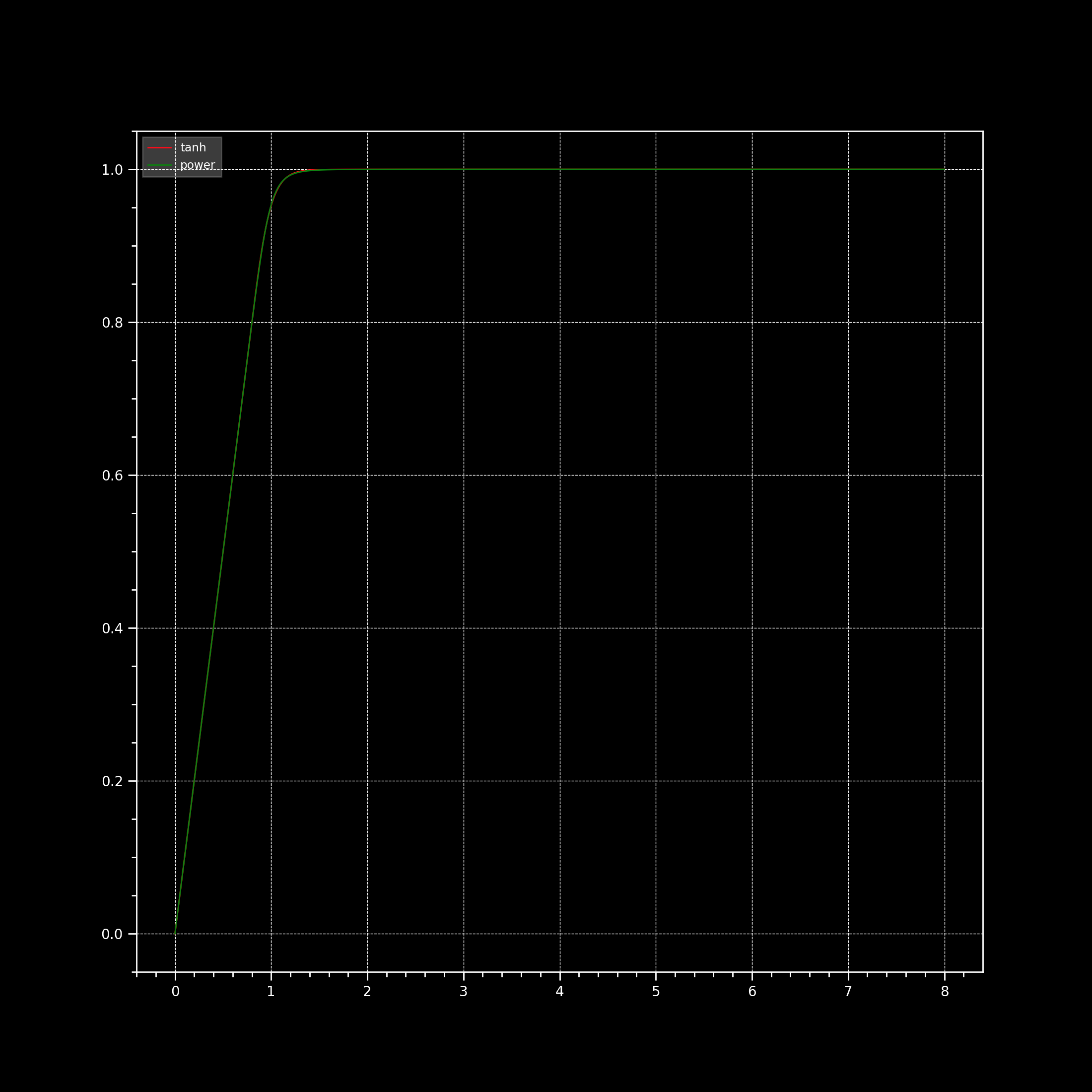
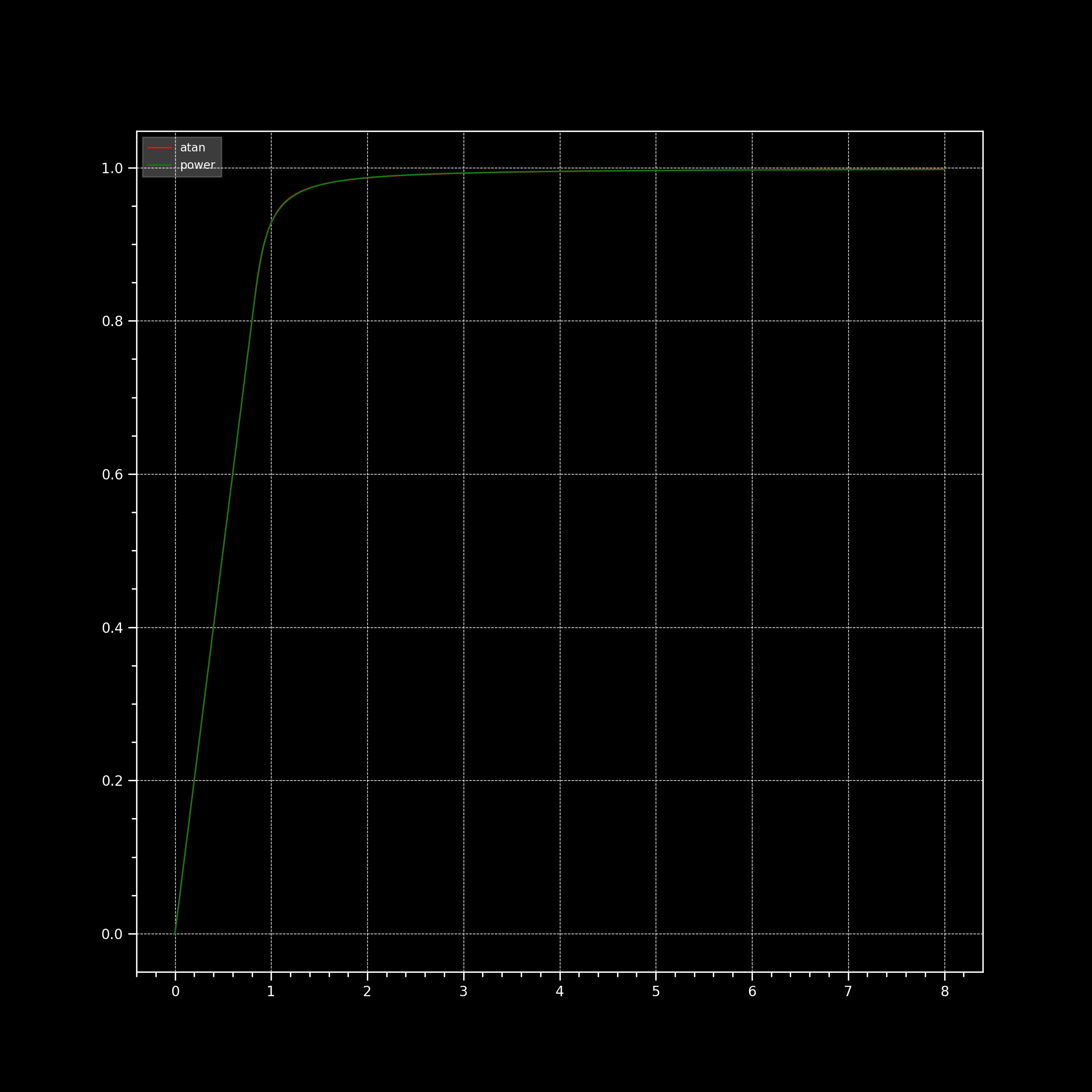
I was fiddling a bit with @JamesEggletonpower function to see if it can fit tanh and atan and it is quite good, not coming as a surprise given the piece-wise power curve above turned to be insanely versatile:
It does make sense to simplify the implementation to a single curve, which by tweaking parameters can be made to closely match all the other candidates. And the removal of the need of the bisection solver is a big plus for it.
The only caveat is that the threshold (1 - threshold as the parameter appears in @jedsmith’s implementation) needs to be dropped to a lower value than might be intuitive in order to match some curves. In @Thomas_Mansencal’s examples above, the “zone of confidence” to match tanh is only 66%. That probably means that some of the more saturated colours in the CC24 are being moved slightly (I haven’t checked). If so, it’s probably negligible, and not visually discernible. But it’s worth mentioning, and getting the group’s thoughts on this before finally deprecating the other curves.
It would be worth checking how much they move though because the MSE is so low, I would be extremely surprised that the difference surfaces visually. We could also compute MSE between 0.66 and the threshold we feel great about.
Oh indeed. I realise I am being pedantic. But we need to check. In the Stated Goals in the Progress Report we wrote ‘Colors in a “zone of trust” should be left unaltered.’ I originally wrote '(or minimally altered) ’ but we decided to delete that.
Yes, I know but if we realise that the MSE between 0.66 and 0.7 or 0.8 is under Half-Float quantization steps for example, it could be considered as unaltered. We expose ourselves, on a daily basis, to alterations in many other places, e.g. forward/reverse matrices defined at 10 places: