RGB Saturation Gamut Mapping Approach and a Comp/VFX Perspective

[jedsmith]

Background

I have been following the conversation about gamut mapping with great interest since it started. I have a feature film vfx perspective on the topic which might be useful. My background is compositing.

In Comp…

In comp the plate is king. All work we do strives to preserve the integrity of the original camera photography. Integration of cg renders, mattepaintings, reconstruction, cleanup etc. In the last few years it has become more common to adopt ACEScg as the working gamut. This approach has advantages. It helps with consistency of imagery from the cg pipeline. It helps with consistency of color pipeline between shows. But it also comes with some problems.

On quite a few shows over the years I have seen the same problem resurface. Highly saturated light sources and flares causing out of gamut artifacts. These negative pixels cause issues for comp. We are familiar with negative pixels in grain and shadow areas, but it becomes difficult to do our work when areas of the image that we need to do work on have this artifact.

I have seen the fallout of a few different approaches for solutions. Leaving the artifacts for comp to deal with can be dangerous and can require a lot of effort to QC comps and support artists. The “Blue light fix” LMT 3x3 matrix essentially shifts the working gamut of the show and can cause problems with cg not matching plates. It can also cause problems when the fix is reversed on delivery, with certain colors getting more saturated than intended. If you’re shifting the working gamut of the show why not just keep the original camera gamut?

Requirements for VFX

In VFX we are required to deliver back comps that exactly match the plates we recieved except for the work we did. For this reason reversing the gamut compression perfectly is critical. However I am acutely aware of the danger of “gamut expansion” as @daniele pointed out. Great care would need to be taken here to ensure things don’t go off the rails.

So to summarize the biggest things comp cares about:
1). Fix the issue so we can do our work.
2). Reverse perfectly so we can deliver our work back to the client.
3). Preserve linearity and hue of the plate as much as possible.

What would it look like?

How a gamut compression tool might be used in VFX is an interesting question. The process might look something like this:

• A 3d lut (applied in the color pipeline / OCIO), possible created with a Nuke node
• Precisely tuned and optimized for the camera gamut and problematic images of the show
• Applied on plate ingest
• Reversed for view transform
• Reversed on plate delivery

A Sketch of a Simpler Approach

All of that said I have been thinking a lot about @daniele’s comment from meeting #8 that the baselight gamut compression algorithm works purely in RGB without the difficulty and complexity of defining the neutral axis.

Given that
1). Cameras are commonly not colorimetric devices (the source of the problem in the first place)
2). Color accuracy is not critical as long as the gamut compression is reversed accurately, linearity is mostly preserved, and hue is roughly correct

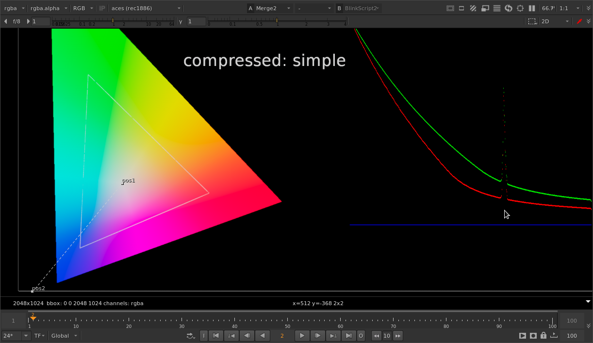
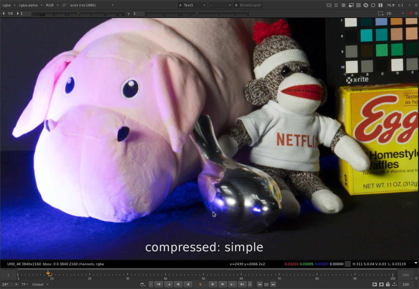
I thought it would be interesting to play around and see what I could come up with utilizing a simple approach of rgb saturation.

Attached is a Nuke script with what I was able to build with my novice color science brain.

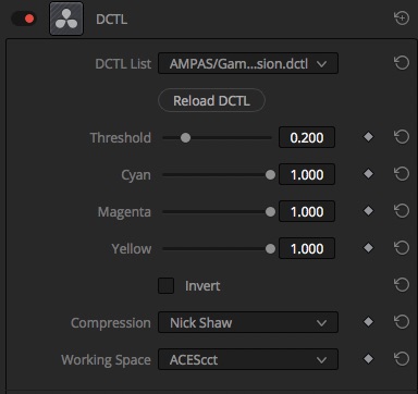
• A saturation algorithm is used to desaturate which is similar to Nuke’s “Maximum” luminance math, but weighted by color channel.
• A core or “confidence” gamut limits the area that the desat affects. The size of the core gamut is set with a threshold adjustment. And the maximum saturation needs to be set (that is, how far outside of the gamut pixels exist, which translates into how far above 1.0 the saturation key goes).

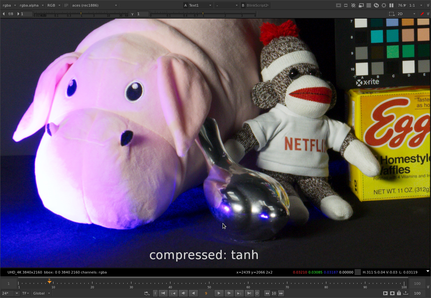
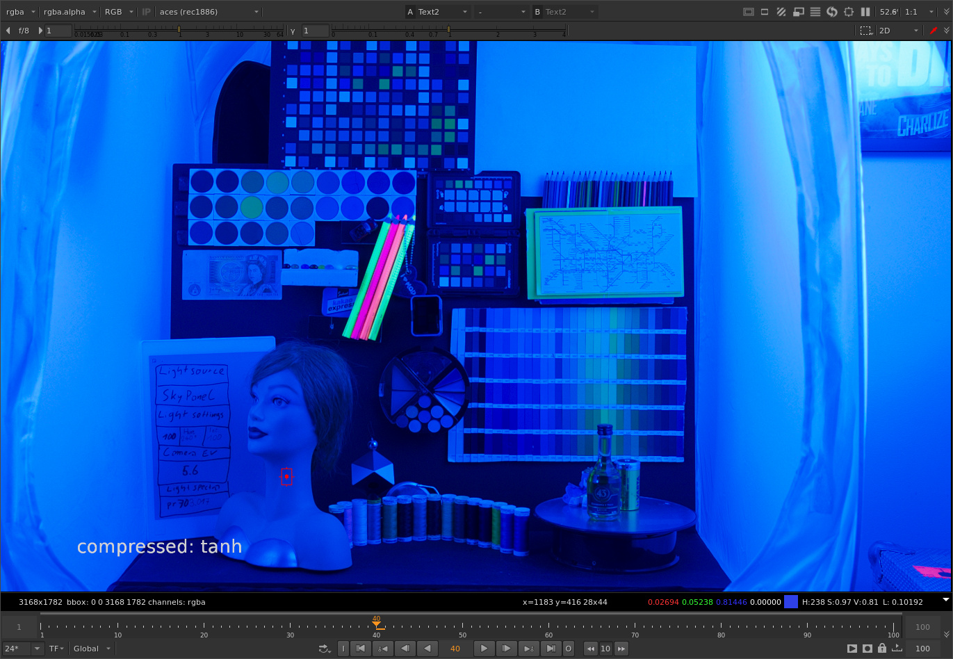
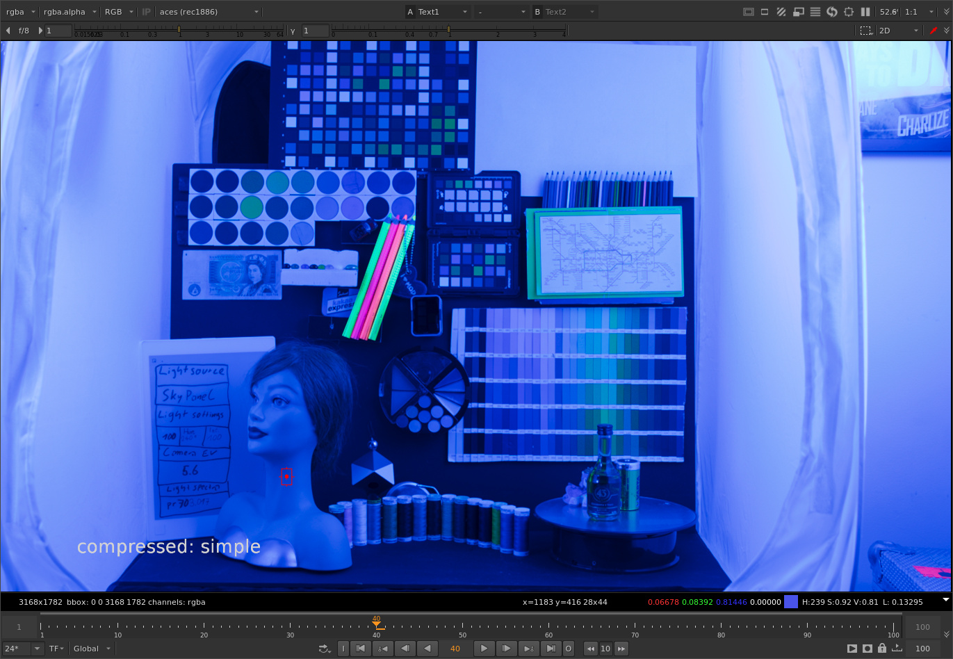
The attached nuke script has a node with a sketch of the idea set up, and keyframes to show the behavior on the example images.

For how simple the approach is I think the results are quite good. It would be great to be able to adjust weighting for the cyan, magental, and yellow directions as well but I have not yet figured out how to do that technically. (Help or ideas would be appreciated here!) Maybe there are other methods of adjusting saturation that would allow more precise control over “color direction”? Or other methods of controlling the direction of the hue vector?

Bonus

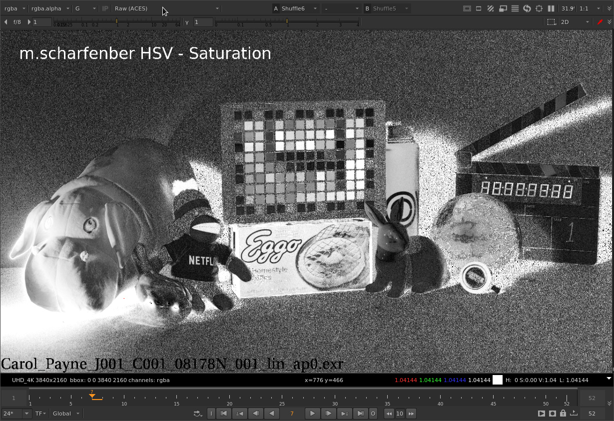
I’ve also included a version of @matthias.scharfenber’s Norm. HSV Sat. Softclip in LMS + Purple Suppression method, with a softclip implementing the function that @nick shared in the Simplistic Gamut Mapping Approaches in Nuke thread - Based on all the testing I’ve done it seems critical to be able to precisely place the start and end of the softclip, and the end may very well not be at 1.0 if there are out of gamut values.

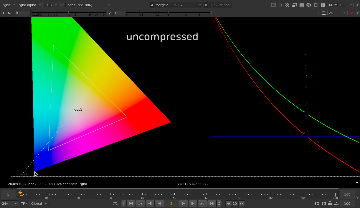
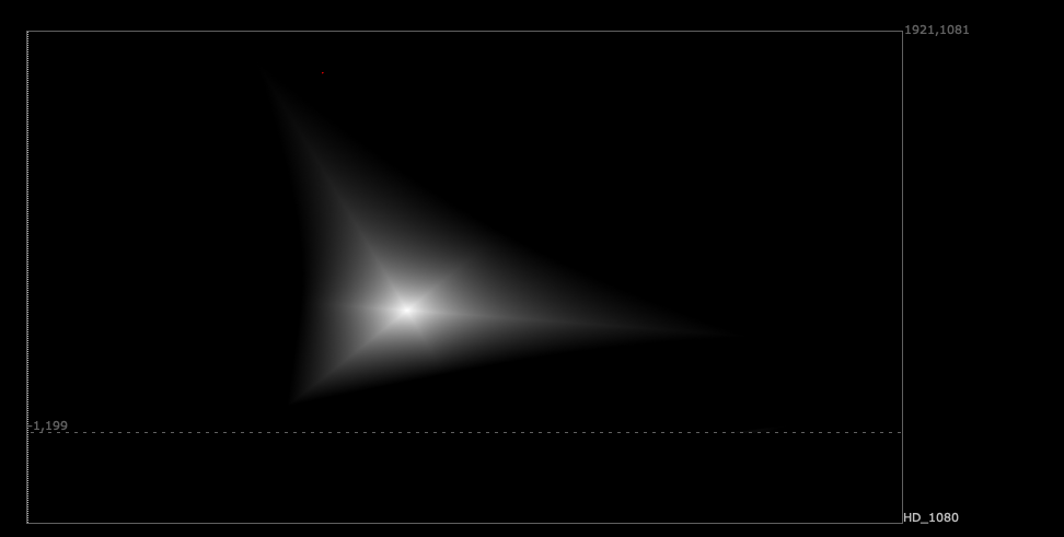
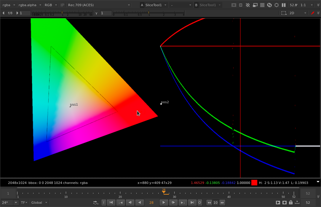
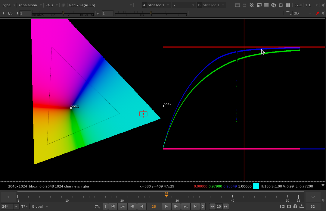
For those of us with a full Nuke license, there’s also a Blinkscript Gamut Plot node, which is less prone to frustrating unresponsiveness than the PositionToPoints + ScanlineRender plotting method.

The nuke script is available here:

https://gist.github.com/jedypod/ea25c5ff2eed68bfeaaafddd26958133

Curious to hear what you all think and sorry for the wall of text!

[daniele (Daniele Siragusano)]

had a look at your nuke script:
Looks quite promising!

I few comments:
Nomenclature:
Luma, Luminance and Saturation are all defined words:

Termlist | eilv

Maybe in our context we could use a few more general terms like Achromatic and Distance instead of Luma and Saturation.

Some thoughts:

• your desaturation algorithm is basically a scale down of the vector {lum,RGB} by the factor saturation, or in other (more general) words you reduce the distance of each RGB position towards its corresponding achromatic position.
• it is a linear fall off meaning two things:
  • 1. the desaturation increases linearly until you reach the outer gamut,
  • 2. once your mask is 0.0 the desat amount does not change
• Calculating the achromatic axis with fixed r,g,b weights will always cause the negative component to bring down the achromatic axis if the negative component gets to small (large negative values).
• some distance function can produce mach bands

here is a screenshot of your distance mask of a xy diagram, revealing possible mach bands

But great job so far!

I hope some of this helps
Daniele

[carolalynn (Carol Payne)]

Hi Jed! Thanks for the work, and for following along with the group. We’re cancelling our next two meetings, but wanted to extend the invite to join the VWG meetings (there are two rotating timezones) if you are able - they are open to all, and we started touching on the subject of invertibility again today based on your post.

Hope you can join!

[jedsmith]

Hey Carol,
Thank you for the invite! Though I do not have the color science knowledge of the others in this group perhaps my practical comp / VFX perspective would be useful.

I guess I missed the last meeting on Thursday, but I’ll try and make it to the next one.

[jedsmith]

@daniele

had a look at your nuke script:
Looks quite promising!

Hey @daniele ,
Huge thanks for the very helpful feedback.

Apologies for the delay in my reply as well, I got distracted by some other projects for the last few weeks and only recently started diving into this again.

I did a lot more work and I think I have something that is headed more in the right direction: Here is a link to a blinkscript code snippet in C++, and a Nuke node. I find the C++ a bit easier to develop and understand what’s going on, but the approach works as an expression node in Nuke as well.

• As Nuke BlinkScript C++ code
• As a Nuke Expression node

Your comment about mach bands and thinking about luminance and saturation as an achromatic axis and distance got me thinking. I did a bunch of research (and learned a lot). I found an interesting paper suggesting a different way of calculating saturation than the typical HSV style cylindrical projection, the IHLS colorspace. I created a Nuke node to convert to this colorspace, thinking this method of calculating saturation might be useful.

Then I realized maybe I was over-thinking the problem even still. Because if we ignore all of the complexities of human vision, camera colorimetry, and all of the complex colorscience that is being discussed in the other threads in this working group, at the end of the day all we need to do is take the pixels that are outside of the gamut boundary and map them back in.

So I thought maybe the distance could be calculated with a very simple Euclidean distance function for each color component. This would specify how far the component is from the achromatic axis. A value of 0 is achromatic, and a value of 1 is at the gamut boundary, and values over 1 are outside of the gamut boundary.

// achromatic axis 
float ach = max(r, max(g, b));

// euclidean distance from the achromatic axis for each color component
float d_r = sqrt( pow(r-ach, 2)) / ach;
float d_g = sqrt( pow(g-ach, 2)) / ach;
float d_b = sqrt( pow(b-ach, 2)) / ach;

With the distance we could now specify a threshold for where the colors would start to be affected.

// gamut compression factor for each color component:
// if threshold is 0.2, 80% of the gamut will be unnaffected
// and the gamut compression will be limited to the outer 20% 
float f_r = max(0.0f, d_r - thr);
float f_g = max(0.0f, d_g - thr);
float f_b = max(0.0f, d_b - thr);

However if we use this as a factor to scale down the rgb vector, it could be pushed more towards the achromatic axis than the threshold boundary, so we need to compensate. We can also add an adjustment for each color component so that we can tweak the “color bias” of the gamut compression.

// scale the compression factor by threshold 
// so that the rgb value is never "desaturated" more than the outer boundary
// limit compression factor by cyan magenta yellow controls
f_r = f_r * thr * cyan;
f_g = f_g * thr * magenta;
f_b = f_b * thr * yellow;

At this point the scale factor is linear, which may introduce mach bands on the edges of the gamut compression threshold. Ideally we would bias the linear factor to have a nonlinear interpolation from the boundary threshold to the outer limit. However this may be over my head mathematically without doing a lot more research! For now I’ve set this up to use a simple gamma power function, which doesn’t look terrible … but is not ideal. Suggestions welcome here!

// apply a power function so that the gamut compression is nonlinear.
// not certain about this approach!
f_r = pow(f_r, 1/cyan);
f_g = pow(f_g, 1/magenta);
f_b = pow(f_b, 1/yellow);

Finally we scale down each color component by the factor and write this out to an image.

// scale down each color component 
// by gamut compression factor towards achromatic axis
float c_r = (r-ach)/(f_r+1)+ach;
float c_g = (g-ach)/(f_g+1)+ach;
float c_b = (b-ach)/(f_b+1)+ach;

I have not yet delved into thinking about how to reverse this process (if inverting is even possible using this approach).

This approach does seem to handle the different sample images better than the last approach I posted. There seems to be much less tweaking of parameters per image required.

Any suggestions for improvements / comments / criticisms are welcome! In addition to any ideas about approaches to nonlinearly interpolating a linear gradient, and thoughts about inverting. Hope this is helpful!

[jedsmith]

I have another update to share!

I spent most of the day working on this and I think I have some good updates.

I spent a lot of time thinking about how to invert the gamut compression and ended up realizing a few things and re-working the algorithm a bit.

The first realization is that the distance function could be remapped directly. Since 1.0 is the boundary of the gamut, and any values over 1.0 are outside of gamut, the distance could be compressed before the scale factor is calculated.

This approach would also theoretically allow the process to be reversed, and for the falloff of the compression to be handled in a more straightforward way.

I’ve updated the same links as before:

• As Nuke BlinkScript C++ code
• As a Nuke Expression node

This update implements @Thomas_Mansencal’s suggestion for using the hyberbolic tangent function as a softclip curve. It works quite well I think. The result is definitely superior to what I had before. There is very little “purple shift” and colors are preserved quite nicely in out of gamut values.

Inverting the gamut compression is kindof working. However, the result is not 1 to 1 because of small differences in the distance function when calculated from the original source compared to when calculated from the gamut compressed source. The inversion of the sofclip curve is working perfectly but since there are small differences in the distance function, those differences get multiplied quite a bit when the softclip is reversed. I’m at a dead-end on this problem for now. The only solution I can think of is to use the distance calculated from the original non-gamut compressed source to use for the “uncompress”, but this is not ideal. It’s possible I’m missing something obvious. Suggestions would be welcome.

I’m also curious to test out some other curves and see if the behavior is any better.

Here are a few pictures to help explain / visualize this highly abstract thing.

This is one of the images I’ve been using to test with. It’s a colorwheel with saturation at 1.75 using “average” mode, plotted on a 1931 xy chromaticity diagram. the gamut is acescg. Here you can see out of gamut values represented in the slice plot on the right as negative values in blue and green.

Here is what the output of the euclidean distance function looks like. As you can see the value for each component is 0 at the achromatic axis, 1.0 at the gamut boundary and is > 1 outside the gamut boundary. Again you can see a slice plot of the values. The bottom red line is 0 and the top red line is 1.0.

And with the compression curve applied with a 0.2 threshold value. This affects 20% of the outside of the gamut.

Here is a detail view of the blue primary without gamut compression:

And with gamut compression applied:

[Thomas_Mansencal]

@jedsmith

This update implements @Thomas_Mansencal’s suggestion for using the hyberbolic tangent function as a softclip curve. It works quite well I think. The result is definitely superior to what I had before. There is very little “purple shift” and colors are preserved quite nicely in out of gamut values.

This is a great function from many standpoints, simple elegance and derivatives among many things, been in my best for quite some years now!

Keep up the good work, I have been continuing some of my stuff over the week-end and I hope to be able to share it this week.

I would like to also try the IHSL paper you linked, yet another HSL model to test! It is much less complex and more elegant than the one I found a few weeks ago.

Cheers,

Thomas

[jedsmith]

Nice! Curious to see what you’re working on.

Yes, the IHLS colorspace is interesting. The complete separation of lightness and saturation is great, and the output of the saturation is much more like you would expect with scene-referred imagery. (No super saturated shadows, handles overbrights well).

Here’s an example comparing it with the old standard HSV model, using Carol’s Netflix monkey image.

[Thomas_Mansencal]

Hi @jedsmith,

Looks great!

Quick question though: are you using Nuke’s built-in HSV model though here? Because it is notoriously bad, I don’t trust it at all and I think it expects non-linear/gamma correct input. @matthias.scharfenber shared some conversion nodes that should be better than Nuke’s node for that!

Cheers,

Thomas

[jedsmith]

Ah yeah good call. Nuke’s HSV was just a particularly horrible image to compare it too

I’ve updated the previous post with @matthias.scharfenber’s HSV implementation, which I should really get into my toolsets. I realized I also had a view transform applied. It’s worth mentioning that the IHLS saturation has a lot of very high overbright values which could be problematic depending on what you’re trying to do.

[daniele (Daniele Siragusano)]

Hi,

Maybe you are the one close to solving this riddle.
I think you are getting there ,
By far, the best approach I have seen in this working group.

I have only a quick read, a few comments though:

float f_r = max(0.0f, d_r - thr);

Because you subtract thr from d_rgb and clamp, and 0 is achromatic, I think the threshold parameter is inverted to what you have described.
so for thr = 0.8 -> 80% of the inner gamut is preserved (because you subtract 0.8 from the distance and clamp to 0).

Here I do not understand why you multiply f_r with thr again.

f_r = f_r * thr * cyan;  

if you remove thr then you see that thr in fact is reversed (see above).

You need to make sure cyan, magenta, yellow factors are below or not much more than 1.0. Otherwise, you get folding, and out of gamut colours could land on a distance smaller than in gamut values.

I am not sure about the gamma function, but you wrote you looked into a different approach.
A straightforward but powerful function to compress values is:

y=x/(x+1)

You can add all sorts of modifier in there too.

So applying your algorithm to AP1, I got good results with this slight modification of your algorithm:

vec4 fn(vec4 val)
{
// achromatic axis 
float ach = max(val.r, max(val.g, val.b));

// euclidean distance from the achromatic axis for each color component
float d_r = sqrt( pow(val.r-ach, 2)) / ach;
float d_g = sqrt( pow(val.g-ach, 2)) / ach;
float d_b = sqrt( pow(val.b-ach, 2)) / ach;

float thr = 0.8;

float f_r = max(0.0f, d_r - thr);
float f_g = max(0.0f, d_g - thr);
float f_b = max(0.0f, d_b - thr);

float cyan = 0.1;
float magenta = 0.5;
float yellow = 0.1;

f_r = f_r * cyan;
f_g = f_g * magenta;
f_b = f_b * yellow;


None linear transformation
f_r = f_r/(f_r+1.0);
f_g = f_g/(f_g+1.0);
f_b = f_b/(f_b+1.0);

float c_r = (val.r-ach)/(f_r+1.0)+ach;
float c_g = (val.g-ach)/(f_g+1.0)+ach;
float c_b = (val.b-ach)/(f_b+1.0)+ach;

val.rgb = vec3(c_r,c_g,c_b);

    return val;
}

We could write this more compact later…

I think it ticks quite a few boxes:

• exposure invariant
• gamut agnostic
• easy to compute
• non-iterative

The inverse should be simple because max(rgb) is not changed by the algorithm.

Great job.
Daniele

[nick (Nick Shaw)]

@daniele

// euclidean distance from the achromatic axis for each color component
float d_r = sqrt( pow(val.r-ach, 2)) / ach;
float d_g = sqrt( pow(val.g-ach, 2)) / ach;
float d_b = sqrt( pow(val.b-ach, 2)) / ach;

I may be missing something, but isn’t taking the sqrt of the square of a single value just the fabs of that value? Shouldn’t euclidian distance be the root of a sum of squares?

[daniele (Daniele Siragusano)]

@nick

I may be missing something, but isn’t taking the sqrt of the square of a single value just the fabs of that value? Shouldn’t euclidian distance be the root of a sum of squares?

yes calling this euclidean distance is a bit misleading, you could call d_rgb inverse RGB ratios…

[daniele (Daniele Siragusano)]

@daniele

f_r = f_r/(f_r+1.0);

oh, just realised that my joined is not monotonic.

[nick (Nick Shaw)]

Is that the reason @jedsmith is multiplying by thr as you commented earlier? This is purely intuitive, so I could be completely wrong, but would normalising back to the threshold make the first derivative 1.0 at the join again?

[jedsmith]

Hey @daniele,
Thanks for the feedback and the kind words!

Sorry for the confusion - I should have pasted my latest code in my last post.

I’ve done a bit more work following your suggestion of a simpler compress function. I’m finding that the rolloff of the compress really has a huge impact on the appearance of the image.

I’ve added a variation on the one you posted, with two parameters: threshold and limit. Threshold is the smallest value that will be affected, and limit is the limit of the curve. This expression is monotonic when l > t and when values below t are unaffected.
t+(-1/((x-t)/(l-t)+1)+1)*(l-t) {x > t}
Here’s a plot of the function if anyone wants to check it out: https://www.desmos.com/calculator/jyewfptd4y

The hyperbolic tangent compress function looks like it has a nicer rolloff on the graph, but I think I prefer the look of images using the simple compress function above.

Here’s a plot of the tanh compress function and its inverse if anyone wants to compare: https://www.desmos.com/calculator/ve9yawvkjf

Here are a couple of images showing what I mean about the simple compress looking nicer.

First this is the source image with out of gamut color values. Again there is a slice plot on the right, and the gamut pictured is ACEScg on an 1931 xy chromaticity diagram.

Next here is the tanh gamut compressed image. The values are mapped into gamut, and there are not artifacts, but the appearance of the out of gamut colors still look very saturated.

Finally here is the “simple” gamut compressed image. The out of gamut colors have a much more pleasing rolloff and the image looks more natural in my opinion.

Here’s another comparison with the Netflix monkey image from @carolalynn - here with the tanh compress function

and here with the “simple” compress function:

And another example from @daniele’s images:
original (in ACEScg gamut)

with tanh compression:

and with “simple” compression:

As before, here are two links to the code:

• Nuke Blinkscript C++ Code
• Two Nuke nodes: a blinkscript node and the same thing implemented as a simple expression node

Inverting the gamut compression is still not working and I’m still struggling to figure out why. My best guess right now is lack of precision, but I have a feeling it’s something else. Any help here would be welcome.

Curious to hear what you all think!

I’ll paste the code here as well so it’s easy to peruse:

kernel GamutCompression : ImageComputationKernel<ePixelWise> {
  Image<eRead, eAccessPoint, eEdgeClamped> src;
  Image<eWrite> dst;

  param:
    float threshold;
    float cyan;
    float magenta;
    float yellow;
    int method;
    bool invert;

  // calc hyperbolic tangent
  float tanh( float in) {
    float e = 2.718281828459f;
    float f = pow(e, 2*in);
    return (f-1.0f) / (f+1.0f);
  }

  void process() {
    float3 lim;
    float cd_r, cd_g, cd_b;
    float atanh_r, atanh_g, atanh_b;

    float r = src().x;
    float g = src().y;
    float b = src().z;

    // thr is the complement of threshold. 
    // that is: the percentage of the core gamut to protect
    float thr = 1.0f - threshold;

    // achromatic axis 
    float ach = max(r, max(g, b));

    // distance from the achromatic axis for each color component
    float d_r = sqrt( pow(r-ach, 2)) / ach;
    float d_g = sqrt( pow(g-ach, 2)) / ach;
    float d_b = sqrt( pow(b-ach, 2)) / ach;
    
    // bias limits by color component
    // range is limited to 0.0001 > lim < 1/thr
    // upper limit is a hard clip, lower limit is no compression
    lim.x = 1.0f/max(0.0001f, min(1.0f/thr, cyan));
    lim.y = 1.0f/max(0.0001f, min(1.0f/thr, magenta));
    lim.z = 1.0f/max(0.0001f, min(1.0f/thr, yellow));

    // compress distance for each color component
    if (method == 0.0f) {
      // softclip method suggested by Nick Shaw here
      // https://community.acescentral.com/t/simplistic-gamut-mapping-approaches-in-nuke/2679/3
      // good results, easy to bias look with limits
      // example plot: https://www.desmos.com/calculator/jyewfptd4y
      cd_r = d_r < thr ? d_r : thr+(-1/((d_r-thr)/(lim.x-thr)+1)+1)*(lim.x-thr);
      cd_g = d_g < thr ? d_g : thr+(-1/((d_g-thr)/(lim.y-thr)+1)+1)*(lim.y-thr);
      cd_b = d_b < thr ? d_b : thr+(-1/((d_b-thr)/(lim.z-thr)+1)+1)*(lim.z-thr);

      if (invert == 1.0f) {
        // inversed compression distance for each color component
        cd_r = d_r < thr ? d_r : (pow(thr, 2.0f) - thr*d_r + (lim.x-thr)*d_r) / (thr + (lim.x-thr) - d_r);
        cd_g = d_g < thr ? d_g : (pow(thr, 2.0f) - thr*d_g + (lim.y-thr)*d_g) / (thr + (lim.y-thr) - d_g);
        cd_b = d_b < thr ? d_b : (pow(thr, 2.0f) - thr*d_b + (lim.z-thr)*d_b) / (thr + (lim.z-thr) - d_b);
      }
    } else if (method == 1.0f) {
      // hyperbolic tangent softclip method suggested by Thomas Mansencal here
      // https://community.acescentral.com/t/simplistic-gamut-mapping-approaches-in-nuke/2679/2
      // gives good results, but perhaps the curve is too asymptotic. very little color shift.
      // example plot: https://www.desmos.com/calculator/ve9yawvkjf
      cd_r = d_r > thr ? thr + threshold * tanh((d_r - thr) / threshold) : d_r;
      cd_g = d_g > thr ? thr + threshold * tanh((d_g - thr) / threshold) : d_g;
      cd_b = d_b > thr ? thr + threshold * tanh((d_b - thr) / threshold) : d_b;
      if (invert == 1.0f) {
          atanh_r = log( ( 1+( thr-d_r) / -threshold) / ( 1-( thr-d_r) / -threshold)) / 2;
          cd_r = d_r > thr ? thr*(-atanh_r) + atanh_r + thr : d_r;
          atanh_g = log( ( 1+( thr-d_g) / -threshold) / ( 1-( thr-d_g) / -threshold)) / 2;
          cd_g = d_g > thr ? thr*(-atanh_g) + atanh_g + thr : d_g;
          atanh_b = log( ( 1+( thr-d_b) / -threshold) / ( 1-( thr-d_b) / -threshold)) / 2;
          cd_b = d_b > thr ? thr*(-atanh_b) + atanh_b + thr : d_b;
      }
    }

    // gamut compression amount: difference between original and compressed distance
    float f_r = (d_r - cd_r);
    float f_g = (d_g - cd_g);
    float f_b = (d_b - cd_b);

    if (method == 1.0f) {
      // directly modify the compression amount by the cmy limits, since the 
      // tanh function doesn't really have a way to rolloff the compression amount
      // maybe there is a way to do this better?
      f_r = f_r * min(cyan, (1.0f+threshold));
      f_g = f_g * min(magenta, (1.0f+threshold));
      f_b = f_b * min(yellow, (1.0f+threshold));
    }

    // scale each color component relative to achromatic axis by factor
    float c_r = (r-ach)/(f_r+1.0f)+ach;
    float c_g = (g-ach)/(f_g+1.0f)+ach;
    float c_b = (b-ach)/(f_b+1.0f)+ach;

   
    // skip black pixels to avoid nan values
    if (r == 0.0f || g == 0.0f || b == 0.0f) {
      dst() = src();
    } else {
      dst() = float4(c_r, c_g, c_b, 1);
    }
  }
};

[Thomas_Mansencal]

Great work @jedsmith! I will try to roll your operator in my notebook to compare with the cylindrical approach.

@jedsmith

Finally here is the “simple” gamut compressed image. The out of gamut colors have a much more pleasing rolloff and the image looks more natural in my opinion.

I think we should probably try to keep the original saturation, and defer (whenever possible) the creative tweaks as a very last step. Shorter roll-off means less effect which is preferable imho, I rarely use x / (x + 1) in production because it tends to be super aggressive and gives less freedom, it compresses values so much that you end up with a super tiny window to tweak things in the upper part of the function.

Cheers,

Thomas

[jedsmith]

@Thomas_Mansencal

I think we should probably try to keep the original saturation, and defer (whenever possible) the creative tweaks as a very last step.

Agreed, and to be fair the tanh function does achieve this better.

Since I’m right at the edge of my math ability, I wonder if you might know of a way to parameterize the tanh function to achieve something similar to this function? Basically being able to specify the limit and the treshold - that is, which number the curve approaches, the “slope” or “aggressiveness” of the curve, and where the curve starts departing from x = y? Or maybe there’s another variation that would be better?

I played around quite a bit but wasn’t able to figure this out with the tanh function.

Thanks for your help!

[Thomas_Mansencal]

Roll-off start is set with a and limit by b: https://www.desmos.com/calculator/uz0if9qc1h, make b free to set the limit to your wish.

[nick (Nick Shaw)]

I have made a Resolve DCTL version of @jedsmith’s BlinkScript. This allows it to run in real-time on moving footage.

nick-shaw/gamut_mapping