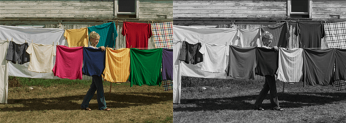
In Part 3, analytic LMTs were introduced by walking through the creation of simple examples. But analytic LMTs can have any number of processing steps, and this post walks through the creation of more complex analytic LMTs.
[Transforms used in this article are again provided as CTL code at the end of the article.]
Analytic LMT – Example 3 (complex)
Example 3 is the probably the most complex example, introducing vector-based secondary color correction and sequencing several independent operations into a single LMT. Structurally, this LMT consists of some primary corrections up front followed by a combination of hue-qualified adjustments to hue angles and saturation. The look was roughly modeled after a print film emulation, resulting in something high contrast and slightly “grungy” (see Figures 16 and 17)*.
[*Please keep in mind that I am not a colorist, and my goal with this look is to demonstrate the possibilities with very complex Analytic LMTs. The result might not be beautiful to you, but it should illustrate the process!]
Design Approach
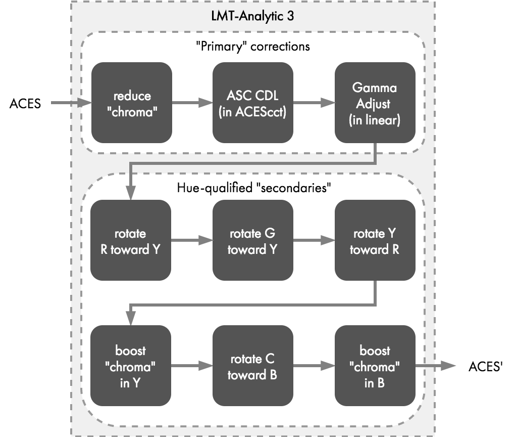
As mentioned, the sequence of operations in the LMT that produced this result is quite a bit more complex than in the previous examples (Figure 18).
The sub-transforms for applying ASC CDL and the gamma adjust are re-used from the previous examples. Each box in Figure 18 is more fully explained in the following sections, with depiction of the before & after with processing up to that individual piece of the processing chain applied.
Introducing “Yab” and “YCH”
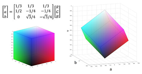
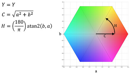
Many of the sub-transforms make use of a a generic lightness/opponent color space, here-in referred to as “Yab.” From Yab, a lightness/chroma/hue representation, referred to as “YCH”, can also be attained. Yab and YCH are defined solely for convenience of targeting specific lightness, hues, or chroma. They are intentionally simple coordinate spaces defined by ratios of RGB and are not intended to have any correlation to perceptual luminance, chrominance, or hue.
Yab can be attained via a simple conversion from RGB; it is essentially a space where an RGB unit cube has been rotated and stood vertically on its [0,0,0] corner such that the neutral axis runs vertically (Figure 19).
YCH is a cylindrical representation of Yab, where C represents the distance of a color from the neutral axis and H is a hue angle in degrees (Figure 20).
Reduce “chroma”
To scale chroma, RGB is converted to YCH, a simple percentage is multiplied to the C channel, and then values are converted back to RGB. Figure 21 shows the before/after of this step, with the chroma scalar value set to 0.7.
ASC CDL (in ACEScct)
The base math for ASC CDL is reused from Analytic 1a and 1b. A fairly minor adjustment to the blue channel slope and offset was made in order to bring a touch more yellow into the overall balance (Figure 22).
Gamma adjust (in linear)
The base math for adjusting contrast with a gamma adjustment in linear was reused from Analytic 1c. Contrast was increased around mid-gray with a gamma value of 1.5 (Figure 23).
Rotate R toward Y
To select hue regions and avoid harsh transitions, a cubic basis shaper function is used. This function tapers from full power, 1.0, at the middle and falls off to zero at a desired width to allow for a narrow to wide range of hues to be affected.
The hue rotation formula takes as input the center hue to be targeted, the width of the hue region to target, and an amount to rotate the hues in that region. Hues that fall at the center location get a full amount of rotation. Hues that are outside of the hue region get no amount of rotation. The amount rotation for hues off of direct center but still in the affected hue region is determined by the cubic basis shaper function.
All of the values chosen were determined through continuous tweaking. Sometimes a pixel was sampled from the ACES image and converted to YCH to determine to what hue it corresponded. A trick to quickly confirm if the correct span of hues is being targeted is to set the hue rotation amount to 180˚, which should have the effect of turning the affected pixels to a hue opposite them on a hue wheel, thus making it easier to identify the affected pixels.
To make reds slightly more orang-ish by rotating toward yellow, the following values were used:
Center hue = 0˚
Hue region width = 30˚
Rotation amount = 5˚
Rotate G toward Y
To make greens more yellow, the following values were used:
Center hue = 80˚
Hue region width = 60˚
Rotation amount = -15˚
Rotate Y toward R
To make yellows just a bit more “golden”, they were shifted toward red with the parameters below:
Center hue = 52˚
Hue region width = 50˚
Rotation amount = -14˚
Boost “chroma” in Y
Boosting chroma in a specific hue region uses a similar tapering function as the hue rotation to again avoid harsh transitions. Values in the middle of the region get the full chroma scaling and the amount of scaling from the original value tapers off to zero at the full width of the cubic basis shaper.
To boost chroma in yellows, these parameters achieved the desired effect:
Center hue = 45˚
Hue region width = 40˚
Chroma scaling = 1.4
Rotate C toward B
Center hue = 190˚
Hue region width = 40˚
Rotation amount = 30˚
Boost “chroma” in B
Center hue = 45˚
Hue region width = 40˚
Chroma scaling = 1.4
And finally, a comparison of the overall before and after:
And applied to a few other images:
More time could be spent matching this LMT more closely to a given PFE, but for general illustrative purposes, this is sufficient.
More complexity could also be added via other qualifying functions. For example, one could create a function to desaturate just shadows (i.e. values with a Y below a certain value). Or a function could further qualify hue regions with both Y and C tapers to only affect bright and saturated, yellows, for example. The possibilities are limited only by the complexity of the adjustment algorithms one can design.
Analytic LMT - Example 4 (complex)
While not as complex as the long chain of secondary corrections used in Example 3, this example recreates the functionality of a node graph with parallel color correction nodes that are mixed together using a given blend mode.
The look approximates that of a “bleach bypass” or “skip bleach”. A preview of the LMT’s effect can be seen in Figures 34 and 35.
Design Approach
The structural model for this LMT was taken from a simple but effective Youtube tutorial wherein creating an easy “bleach bypass” or “skip bleach” using blended node corrections is described.
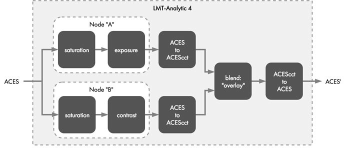
The processing chain is illustrated in Figure 36. Two copies are made from the input ACES2065-1 data. The first copy is desaturated slightly and increased in exposure. The second copy is fully desaturated and boosted in contrast. The two modified copies are then mixed together (in ACEScct) using the “overlay” blending mode.
Node A
Saturation (in linear)
Saturation is slightly reduced using a 3x3 saturation matrix with the saturation factor set to 0.9.
Exposure (in linear)
Adjusting exposure in linear is achieved by multiplying by a scale factor. In this example, a good scale factor was determined to be 2.0, which represents a doubling of exposure.
Node B
Saturation (in linear)
Saturation is slightly reduced using a 3x3 saturation matrix with the saturation factor set to 0.0.
Contrast (in linear)
The math for adjusting contrast with a gamma adjustment in linear was reused from Analytic 1c. Contrast was increased around mid-gray with a gamma value of 1.2.
Blend
The resulting images from Node A and Node B are compositing using the “overlay” blend mode. In the CTL example, this operation is performed in ACEScct, so there is a conversion from ACES2065-1 to ACEScct prior to the overlay blend and a conversion back to ACES2065-1 from ACEScct after the overlay blend.
And applied to another image:
Supporting CTL transforms
Below are download links for the CTL transforms used in the examples in this post.
- Analytic LMT 3 : rough “PFE-like” look (high contrast / grungy) using sequenced hue-qualified adjustments
- Analytic LMT 4 : “bleach bypass” look using overlay blend mode
Dependencies:
- Current release of aces-dev
- ACESlib.LMT_Common : provides various subfunctions used throughout the analytic LMTs
Notes on LMT implementation
The transforms used in all examples are provided as CTL code. LMTs do not need to be implemented in CTL. CTL was the easiest way to unambiguously express the operations used. If you are a “tinkerer” feel free to take a closer look at the formulas inside the CTL for the order of operations and other details on how these LMTs work.
The Common LUT Format (CLF), a core component of ACES 1.x, is designated as the official carrier for certain kinds of LMTs. CLF’s can encapsulate any number or ordering of process nodes that include 1D LUTs, 3D LUTS, matrices, and ASC CDL. However, CLF does not support math formulas, so CTL used for even simple shaper functions would need to be sampled to LUTs for implementation in CLF. This is potentially limiting, but extending CLF, or adding support for algorithmic description of LMTs, is under consideration for upcoming ACES enhancements and extensions.
Please note that CLF is a required item for LMT-supporting production and postproduction tools that wish to achieve the ACES Logo. We encourage all end-users to work with ACES Product Partners to provide you with this powerful capability.
Regarding LUTs, keep in mind that the quality of 3D-LUTs requires knowledge of input and output ranges as well as grid point spacing. ACES values are radiometrically linear and have a very wide floating point range. Spacing nodes directly in linear space does not always provide a good sampling of the useable range. CLF provides for forward and inverse ‘shaper LUT’ operations that (when wrapped around an appropriately constructed 3D-LUT) can effectively produce well-spaced LUTs with minimal interpolation errors. Implementers should review the ‘1D LUT’ section of the Common LUT Format specification [S-2014-006] for more information.
Where to go from here
With the “nitty-gritty” of what goes into and how to build LMTs described in Parts 2-4, one can see that both empirical and analytic LMTs are not always terribly difficult to make. Once constructed LMTs can be a valuable tool for those using ACES for their color pipelines.
LMTs are basically “preset” looks, and one may find it desirable to build up a library of pre-built filters that can be used to quickly decide a look that fits the project.
To hone in on the types of operations you might need to achieve a look, toying around with a color corrector’s operators can be useful. Of course each color corrector likely implements different math for its secondary operators and hue-specific adjustments, etc. but it can be helpful for look designers to at least determine what regions need to be targeted and in what direction they need to be adjusted.
Experiment on your own and try using LMTs to implement your own looks. Your ACESCentral friends would love to see what you come up with. Feel free to extend the provided functions or write additional ones. In this spirit, a few more creative looks will be posted in the coming weeks.
Questions and comments below!


