Output Transform Tone Scale

Except it is a different medium to film, no? What does a “tone” mean here? Is it somehow different to the double duty that a density plot represents with film?

It’s a shifting nonlinear result underneath a nonlinear curve. This would seem to make it nearly impossible to comprehend the meaning of the curve in question, given the plot is nonlinear that it is on top of?

Yes, in the perfect world with no performance, energy or bandwidth constraints, the EOTF is not required, e.g. a full floating-point display chain. Generally best to leave it alone and think about it as a no-op even though it is not necessarily strictly the case. Put another way we do have an EOTF mostly for (good) cost reasons.

2 Likes

Very interesting point. I always felt that something like this was going on but never dared to ask. Thanks for having clarified this topic !

3 Likes

I have been doing a bit of research and experimentation in the domain of tonescales. Specifically, simpler formula-based alternatives to the spline approach used in the ACES SSTS. Full disclosure, I’m embarked on this adventure partially because I am too dumb / don’t have the knowledge yet to implement splines myself. And I find their complexity a bit overwhelming, and have the gut feeling that there are simpler alternatives.

I will share here a few things I made along the way in case anyone finds it interesting or useful.

Hable Piecewise Power Tonemap
One of my first experiments was diving into John Hable’s Piecewise Power tonemap, which was discussed previously by @Thomas_Mansencal. I was intrigued by the (relative) simplicity of the piecewise power curve fitting, but I didn’t really understand how it worked on a mathematical / technical level. So I decided to implement it myself starting from scratch.

Above is a link to a desmos implementation. I have changed the parameterization a bit from what is proposed by Hable. The parameterization expresses

  • The linear section pivot as an xy coordinate
  • The slope of the linear section
  • The shoulder and toe linear section length
  • The shoulder asymptote position as an xy coordinate
  • The toe asymptote position as an xy coordinate (Note that the Hable implementation assumes a 0,0 coordinate at the origin, and is thus a bit less flexible).

I also added an inverse transform based on the same parameterization.

This s-curve would be applied in a log domain.

There is a Nuke implementation here, and a blinkscript version here.

The big downside of this curve is that it’s not possible to control the slope or behavior of the shoulder, and the shoulder tends to compress values too much as it approaches asymptote. One can work around this by adjusting the shoulder asymptote xy position, but it’s tricky and doesn’t work super well.

PowerP Sigmoid
Frustrated by the Hable shoulder, I decided to embark on an adventure in math to make my own parameterized sigmoidal curve using the Power( p ) compression function that @JamesEggleton posted here. After a couple of weekends learning calculus I finally figured out the math to solve for the intersections, and made this:

  • It has similar parameterization for the pivot, and toe / shoulder linear section length.
  • Has “power” adjustments for both shoulder and toe compression curves.
  • Has a solve for shoulder limit and toe limit, to specify what x value crosses y=1 and y=0.
  • Has an inverse, (it’s a little buggy in the desmos implmentation but the nuke version works okay)

Note this is pretty similar to the tonescale in the NaiveDRTPivoted node, but all combined into one transform instead of being separate pieces.

The curve is very flexible, but unfortunately I wasn’t very happy with how it looked. I really struggled to get the curve for shadows to look good in images.

Here is a Nuke implementation, and a Nuke implementation applied in the log domain.

Hill-Langmuir Equation
I got distracted into implementing a few more color models in my growing collection, and read Fairchild’s HDR-IPT paper. It mentioned the Michaelis-Menten model of enzyme kinetics used in biochemistry as a way of describing the human visual system response to increasing light stimulus. This is also discussed a bit in the Kim / Weyrich / Kautz 2009 siggraph paper Modeling Human Color Perception under Extended Luminance Levels. I was very curious about this curve because it has almost the exact shape of 1D lut component of a print film emulation lut, and many show luts I have encountered over the years. I was also particularly interested in this curve because of how insanely simple it is.

I chose to use a variation of the Hill-Langmuir formulation, because it provides a bit more flexibility. I solved for the inverse, solved for the y=1 intersect.

I also did a variation with a linear extension on the toe and shoulder, but later thought I probably didn’t need this.

The Hill-Langmuir tonescale is the one I’m using in my OpenDisplayTransform project.

Nuke implementation with the linear extensions available here, and a simpler version with a log-domain wrapper available here.

Timothy Lottes
I also implemented the Timothy Lottes 2016 Tonemap Operator (and display rendering method). It is a nuke node available here.

Others
I also tested like 20 other sigmoidal type functions if anyone wants to play around with them, they are all here.

Edit - Just wanted to put a link to a desmos plot of probably the top “honorable mention” sigmoid - the 4-parameter logistic curve:

11 Likes

thanks for this:

Here is another one:
It takes scene-referred linear whatever :wink: and outputs display-referred linear whatever :wink:
It is already formulated so it can be directly applied to images and addresses the whole SDR/HDR problem space.
It is the most simple form I could think of, and it could be expressed in actual a single line instead of the two lines rendering code (which I added for readability).
Invertablitiy is trivial.
It is based around the Michaelis-Menten equation.
It has a gamma model for surround compensation as well,
If you look at it in desmos it does not look like a typical sigmoid, this is because Desmos does not have log ranging axis.

8 Likes

This is so elegant and simple it makes my brain hurt. Thanks so much for sharing this @daniele!

After a lot of fiddling about, I managed to figure out how to fake a log-plot on the x-axis on desmos (I made a simple acescc function with x stops above and below 0.18, then ran the functions through that).

As usual, I can’t understand anything until I implement it as a Nuke node… so here’s a rough implementation of your math if anyone wants to experiment with it.

EDIT updated to fix bug with blue channel, and including inverse
ToneCompress.nk (2.2 KB)

Also as usual, I’m gonna swoop in with some stupid questions.

Over the weekend I did some reading on HDR, trying to learn a bit more about it. I read ITU-R BT.2390-8 and ITU-R BT.2100-2 among a few other things. I still don’t feel like I have a good grasp of the rendering side of it.

So, stupid question number 1:

  • If you specify peak luminance in nits, is there any reason why normalized white would be different than peak luminance? Are there certain variants of HDR (all?) where these two should be different? To phrase the question another way: Should peak luminance be mapped to display linear 1.0 always, or not? (Maybe this has to do with the inverse EOTF?) (Maybe this is a useful parameter to limit the max luminance? Say if you wanted 600 nit peak brightness on a 1000 nit display?)
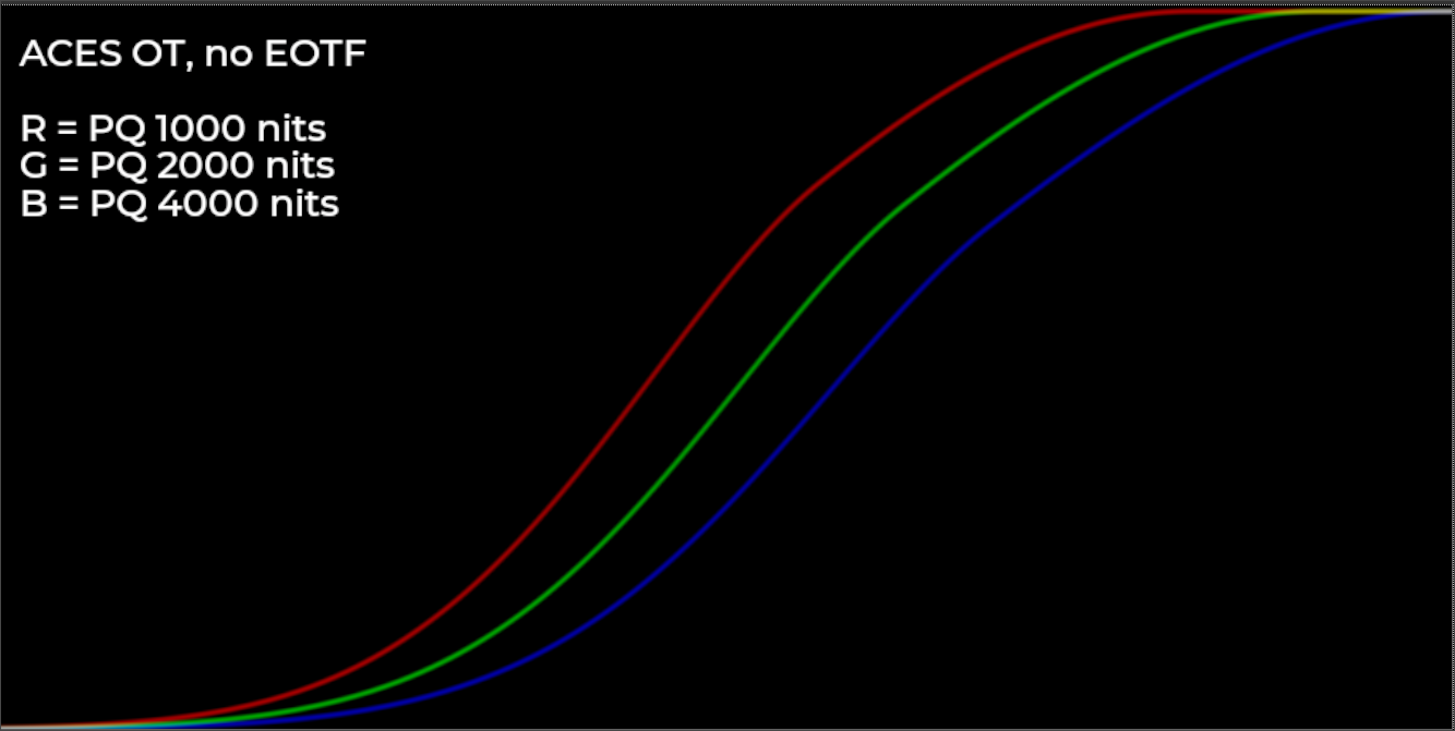
    If I interpret the ACES Output Transform correctly (this being my only open-source reference point for HDR display rendering), it looks like the only difference between the 1000, 2000, and 4000 nit variants of the Rec.2020 ST-2084 PQ HDR Output Transform is an exposure offset of the tone curve, similar to what the “Exposure” adjustment in your equation does. (Although I might be missing something here).

Stupid question number 2:

  • Do you feel that a simple power function is sufficient for surround compensation? I spent a while digging around in papers from the 1970s trying to find the actual math for the Bartleson-Brenneman equations, which you mentioned in one of your talks for Filmlight… But I was never able to implement it fully to compare with the (seemingly) more common power function.

Stupid question number 3:

  • When you boost the shadow toe flare/glare compensation, it lowers the asymptote of the curve by the same amount. Is this by design, or is there a normalization factor to counter this toe adjustment missing?

Finally, a few naive observations:

  • It is super interesting from a simplicity standpoint to not have to wrap the a sigmoid in a log domain transform and then jump through a bunch of hoops to go back and forth between linear and log domains.
  • It is really helpful (at least for me) to see what a proper parameterized formula-based implementation might look like. I’ve been shooting in the dark a bit with my experiments, and this is useful to shape my thinking (in addition to being just plain useful).
4 Likes

Hi,

Some comments on your questions:

Q1)

  • normally you want to establish a common metric in both input and output domains, the normalised white helps with this.
    If you would choose luminance as the output domain you could define 1.0 as 100 nits so 10.0 would be 1000 nits etc…
    How you translate then the scene-referred image into that specified output domain is again another topic.
    But the normalised white is kind of the anchor point of this consideration.

Q2)

  • Works great and it is super simple.

Q3)

  • I did not bother putting t into the calculation of m because it is a tiny nudge in white really - so it is not visible, but of course, you could say m=\frac{n}{n_{r}}+t . This would correct for t in peak white roll-off. In practice, you choose n a bit brighter than the actual display peak so that you run into the peak with a finite scene-referred value.

Glad that you find it useful.

5 Likes

In HDR, normalized white usually means reference white so around 107 nits in original Dolby PQ documents or 203 nits in updated ITU BT. 2408-3 (must read) which tries to match PQ levels with HLG levels for broadcast. Protip: when blending SDR display referred logos and menus over tonemapped HDR, you want to scale the max white of your original SDR content to a bit brighter (between 1.25x and 1.5x) than the HDR reference white you’re using since you want your logos and menus to visually pop.

Peak luminance in nits is an absolutely crucial parameter to have given the state of HDR PC monitors (shots fired at DisplayHDR 400 monitors and those who buy them). When switching to HDR mode, we use this to calibrate the tonemap curve to the user monitor. As for lower nits sim on a higher nits monitor, it is just a matter of adjusting the calibration parameter when using a configurable tonescale curve. Of course, it’s also possible to clip the display referred output if the goal is to preview what a cheap monitor with a clipping internal display mapper would do with the output from an uncalibrated tone curve.

That’s because middle gray in SSTS is calculated to land at 4.8 nits before exposure offset. The exposure offset is calculated based on the parameter which allows to set where middle gray lands. All of the ACES reference HDR curves have it set to land at 15 nits so the differences you’re seeing here are related to the interpolation between the SDR curve and the RRT curve.

That is what scRGB does except that it defines 1.0 as 80 nits and 12.0 as 1000 nits. The problem is that it takes the narrow view that SDR reference white is the correct one to have. The whole debate between 107 nits reference white PQ and 203 nits reference white PQ is a cautionary tale. BT. 2408 adds a further twist and says that 203 nits is only correct when the peak luminance of the mastering display is 1000 nits. For higher or lower peak luminance, reference white should be adapted accordingly.

1 Like

I guess you miss understood,
The reference white is just a concept to align various DRT from one family. It just defines the output scale. It does not define how and where you map scene-referred data to, this is defined by the DRT itself.
And I agree, the debate about mapping grey or diffuse white is somewhat misleading…

1 Like

Well, my answer stems from the fact that our current SSTS outputs values in cd/m^2 and I find that very useful so my preference go to keeping it that way. Alright, when using it for SDR, the output has to be remapped to relative 0…1 and any kind of units work since the remapping formula removes the unit (which means they could even be meatballs :slight_smile: ).

well you need to rescale for any inverse EOTF ]. PQ for example defines 1.0 at 100000 nits. If you want linear light display values directly in cd/m2 you put reference white to 1.0.
So your preference is one particular setting in the more general framework I have suggested.
It is even more useful if you start with cinema viewing condition where you actually want to map what was previously on 100 nits onto 48 nits or vice versa, but without changing the shoulder.

2 Likes

Ah I see where the confusion comes from. For me, HDR reference white is not peak nits but diffuse white (I used to call this paper white but I switched after reading BT.2408-3). Basically the output value of ssts(1.0). I do not consider the inverse EOTF (or the OOTF in the case of HLG) at this point. Instead, my only consideration is: where do I want this to land in absolute land and I can validate this by doing a straight InversePQ(value / 10000) without any further processing.

Here’s the quote from which I take my definition:

The reference level, HDR Reference White, is defined in this Report as the nominal signal level of a 100% reflectance white card. That is the signal level that would result from a 100% Lambertian reflector placed at the centre of interest within a scene under controlled lighting, commonly referred to as diffuse white. There may be brighter whites captured by the camera that are not at the centre of interest, and may therefore be brighter than the HDR Reference White.

Graphics White is defined within the scope of this Report as the equivalent in the graphics domain of a 100% reflectance white card: the signal level of a flat, white element without any specular highlights within a graphic element. It therefore has the same signal level as HDR Reference White, and graphics should be inserted based on this level.

Only for achromatic R=G=B. For everything else it’s a skew.

I agree 100% that it’s a skew since we evaluate it per-channel and that brighter saturated colours have it worse. The stated goal though is to have a float3 vector which gives the expected output in absolute luminance if the display gamut was AP1. Given that we need to perform AP1->Display gamut conversion then it’s more like a rough idea but it remains useful enough that I’ve been able to fake a SDR from the PQ output of the HDR transform without inverting everything. I only used PQ->Linear, a few rescale, clip and gamma operations, Bt2020->Bt709 followed by more gamma adjustments (sRGB monitor curve folded in the lot). Why? XBox GameDVR obligé :slight_smile:

Just a quick post to say that I’ve updated the “ToneCompress” nuke node in my post above.

  • I successfully worked out the math for the the inverse transform. (making progress huh? :smiley: Couldn’t have done that a year ago!)
  • I fixed a bug with the blue channel
1 Like

Anyone tried fitting the current HDR transforms with the Michaelis-Menten inspired curve?

This weekend I’ve spent some time more deeply examining the math of the Michaelis-Menten style compression function that @daniele posted. I have a few useful observations and discoveries which I will share here.

I think it is useful to split apart the compression function into discrete components. I keep going back to the simplicity of my first prototype NaiveDisplayTransform. In that prototype it was very easy to calculate a gamut volume compression as display referred output approaches display maximum, because the “shoulder” compression was an isolated operator. In psuedocode,

norm = max(r,g,b)
shoulder_compress = compress(norm)
factor = 1 - shoulder_compress / norm
factor = pow(factor, bias)

factor is then the factor for the lerp towards 1.0 in the rgb ratios. Super simple, and looks better than the hacks I’ve been doing in my last versions of the OpenDisplayTransform where I am using some power bias of the compressed norm as the factor.

But for this approach to work, shoulder compression must be separated from the other components of the compression.

So! I started digging in to the math of Michaelis-Menten. Daniele’s compression curve is a combination of 4 main things:

  • A normalization factor (basically a multiply).
  • A shoulder compression to accomplish highlight intensity rolloff.
  • A power function to adjust contrast and do surround compensation.
  • A toe compression to do flare compensation.

Shoulder
The shoulder compression function is the first thing I started digging into. While implementing my Hill-Langmuir sigmoid compression function, I remember reading in the wikipedia article about it that the Hill-Langmuir equation is a special case of a rectangular hyperbola.

In fact, when n=1 in the Hill-Langmuir equation, the function is a rectangular hyperbola. In it’s simplest form a rectangular hyperbola is the function f\left(x\right)=\frac{1}{x}

When n=1 in the Hill-Langmuir equation above f\left(x\right)=\frac{x}{x+1} Does this look familiar? Yes, it’s a “simple Reinhard” compression function, which is a hyperbola that is offset such that it passes through the origin.

What is super super interesting about these curves however, is how they look on a x-log, y-linear plot. Spoiler: It’s a sigmoid!

Here is a desmos plot showing this:

Toe
So what happens in the Hill-Langmuir equation above when n>1? We are increasing the strength of the toe compression. I didn’t understand this until seeing it split apart in Daniele’s compression curve, but the function is a skewed parabola: f\left(x\right)=\frac{x^{2}}{x+a}

I got really fascinated by this function because I’ve never really seen parabolic functions used in image processing before, and they have a number of very interesting qualities:

  • Exponential (parabolic?) increase in compression as the x value approaches the vertex of the parabola.
  • Pretty much linear beyond a certain distance from the vertex.

Parabolic Compression Function
So I spent a few days reading about and playing around with Conic Sections and Parabolas, which I haven’t really investigated since highschool many years ago. One super interesting form of this function is as follows f\left(x\right)=\sqrt{2cx+\left(j^{2}-1\right)x^{2}}, where j is the eccentricity and c is the slope.

Depending on the eccentricity, it smoothly transitions form an ellipse to a parabola, to a hyperbola. Pretty crazy! :smiley:

Then I got to thinking… (Can you tell I’m really good at getting side-tracked?). Maybe this parabolic function could work really well as a compression function. Back in the gamut mapping virtual working group, the compression function which I liked the look of the most was actually the log compression function. Something about having a more linearly increasing slope over the compressed area, to distribute compressed values more evenly, helped preserve more tonality in affected regions.

This is the desmos plot of that log function

Of course the problem was that there was no closed-form solution for solving for the y=1 intersection (at least not that I could find at the time).

So I spent a little while investigating if there could be a way to create a parabolic compression function which operated in a similar way. It took me a while but I figured out the math to do it. I’ll link desmos plots of my process below in case anyone is interested in this stupidly nerdy stuff:

And finally, in simplified form, with solution for intersection constraint:

f\left(x\right)=\left\{x\ge t:\ c\sqrt{x-t+\frac{c^{2}}{4}}-c\sqrt{\frac{c^{2}}{4}}+t\right\}

where c is the calculated scale factor based on some constraint coordinate which the function must pass through: c=\frac{\left(1-t\right)}{\sqrt{\left(l-t\right)-\left(1-t\right)}}, l is the x coordinate at y=1 that the compression function must pass through, and t is the threshold at which compression starts.

I literally just figured this out so I haven’t really tested it yet, but I’m super curious to see how it works for gamut mapping distance compression.

As usual here it is as a nuke node as well:
CompressParabolic.nk (2.7 KB)

I’ll stop rambling about nerd stuff now. Just wanted to share some of the things I’ve been up to in case anyone is interested or finds this useful! :slight_smile:

6 Likes

Why do you need to split this all up?

I suppose I do not have a good reason to split all of the different pieces up into individual operations (besides this making it easier for me to understand more completely).

I guess the only valid reason is to get access to the shoulder compression in isolation from the other steps for the “path to white” factor, which I mentioned above. Although perhaps this is invalid as well, if I’m missing something obvious. (Quite possible).

1 Like

Several years ago now I had investigated a few of these functions for use as a tonescale (although you have presented quite a few more than I remember). The problem I always encountered was that if I adjusted one part of the curve, too much of the rest of the curve changed. So, for example, if I had the position and slope of mid-gray where i wanted it but then tweaked the shoulder ever so slightly, it would affect both the midpoint and max point slightly. I wanted exact control over each key point that I cared about - and I didn’t want to set a value where I liked it and then need to go back and retweak the parameters if I changed a different value. It was infuriating and felt like pure trial and error curve tuning.

This is one of the reasons I eventually resorted to the SSTS, which is two B-splines joined intelligently at the mid point. It offered me exactly the control over the key points I wanted - the min, mid max locations and slopes, as well as the “sharpness” of the bend between min-mid and mid-max.

I’m saying this mainly for context and not trying to say B-splines are the only solution and I have been thorougly enjoying your posts and explorations into other curve options, @jedsmith. If you can find a solution that works and is simpler than the SSTS that will be fantastic.

5 Likes