The recording and notes from meeting #155 are now available.
From the meeting notes, @KevinJW said:
Also the chroma compression and gamut mapper both use the reach limit, but one is nominally source parameters related and the other is nominally output parameters related. At the moment the model parameters are the same for input and output. But if somebody wanted to change that, each reach gamut should use the appropriate parameters.
I think the reach tables for chroma compression and gamut mapper are and should be exactly the same. And the purpose why the table is what it is is also the same for both. The purpose is to reach out to a point what would be equivalent to AP1 boundary in chromaticity space, so that when we invert we can get back to AP1 in chromaticity space.
That is also the reason why both chroma compression and gamut mapper (in getReachBoundary) uses model_gamma to scale the reach M value, as that’s what the model itself uses when going back-and-forth. If we didn’t use it, the reach value wouldn’t be equivalent to AP1 boundary, it might be inside or outside AP1.
There should be no difference between the reach tables generated for chroma compression and gamut mapper, and we should have only one reach table. The following two lines in the code should produce two identical tables. We should remove one of them.
    initialise_reach_cusp_table(cgamutReachTable, gamutCuspTableSize, limitJmax, inWhite, XYZ_to_RGB_cgReach);
    initialise_reach_cusp_table(gamutCuspTableReach, gamutCuspTableSize, limitJmax, inWhite, XYZ_to_RGB_reach);
The reason why we have two different tables is that we have the option to change the chroma compression space. But we chose that both chroma compression and gamut mapper reach would use AP1, so we don’t need different tables anymore.
So there should only be need for three different tables: AP1 gamut cusp table, AP1 reach table, and the limiting gamut cusp table.
1 Like
Sure, but that then means using the display based model parameters and so the actual space is not exactly the same as the input being AP1, different display transforms could modify this. Not a problem today when all the parameters are matched between the two, but it is like a hidden bug waiting to cause issues in the future if we don’t clarify what it should be.
1 Like
Then we just need to clearly document the restricted form and parameters of the model that the DRT is intended to work with.
In an ideal world it might be nice for e.g. OCIO to generalise all the functions that make up the DRT, such that you end up with a selection of fixed functions that can be used as a toolkit for other Hellwig based processing.
But my response to that would be to say firstly that our remit was just to produce a DRT, not to make a DRT from a Meccano kit of parts that would also be useful to other people for doing other things. And secondly that runs counter to @doug_walker’s desire to simplify the code. Something which is hard-coded to do only what we need is going to be inherently simpler than code which retains flexibility to be used differently.
An example of the different “conditions” fed into the model would be the chromaticities/white point which are used for the calculation of the reach table, this would ‘logically’ be source referred as it is AP1 and we want it to be “the same” for all outputs, yet strangely we also use the peak luminance which obviously varies.
Currently the CTL calculates them via two different means make_gamut_table() and make_reach_cusp_table() e.g. aces-output/rec709/Output.Academy.Rec709.ctl at main · ampas/aces-output · GitHub which potentially results in the tables not being identical across all hues.
Separately I’ve also experimented with setting up the XYZ<->JMh with clearly defined source vs display conditions as well as trying to sample everything on the same hue slices, it was this that made me aware of the potential discrepancy between a JMh space defined with different conditions, under those circumstances they are not strictly the same JMh values, or at least you don’t end up with the same reach boundary [edited}
This is the kind of difference that I have between a JMh space with an ACES vs D65 white point, all else remaining the same (showing this because I can easily generate it)
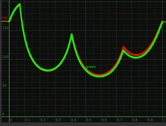
In the gamut mapper where we are doing things relating the display gamut with the reach boundary I’m not clear in my head what the consequences are.
That’s because the table includes the (non-scaled) M value at limitJMax. Should it not be possible to derive the 100 nits equivalent reach M value from a 1000 nits (or 10000 nits) equivalent reach M? Edit: I haven’t tested the following but I think it is:
M_{100nits} == J_{100nits}^{\frac{1}{cz}}* M_{10000nits}
And that is what happens, in Blink as well. It’s two different lookups, though. I agree it’s a bit strange, but we never went on the journey making all the tables have same spacing.
But we don’t use D65 in reach mode. The reach mode operates always, in gamut mapper as well, with ACES white point (as it’s AP1). If the white point of the reach table is changed it won’t invert exactly to AP1 boundary (we had that bug not long ago).
Sure the reach JMh is based on an ACES reference white, but the gamut compression display gamut is generated with a display white reference.
In the CTL the reference white is calculated here aces-dev/lib/Lib.Academy.OutputTransform.ctl at v2-dev-release · ampas/aces-dev · GitHub this gets called with difference matrices wiith different embedded white bal;ances that is what results in the difference in my plot.
So when we compare the display’s JMh vs the reach JMh they don’t exactly mean the same thing.
I went through that experiment. It’s close, but it doesn’t exactly work, because the ‘seam’ down the edge of the gamut volume at a given primary or secondary is not at a consistent hue as the J value decreases. You would get approximately the right answer, but the accuracy would decrease near those corners. We would be making a decision to add another level of approximation for the sake of simplicity. Would we want to make that tradeoff? It think @KevinJW’s idea of storing multiple values at the same hue samples is probably a less damaging tradeoff.
I may be wrong, but I don’t see that as a problem. I see the JMh space as a ‘connection space’ between the two, abstracted away from either white point, because the transform in or out of it includes a white adaptation.
The reach boundary that we pull from is related to the source, and therefore should be calculated using the source RGB to JMh transform, white point and all. We then compress to a volume in JMh calculated based on the limit, which is what is ‘going to happen’ to the JMh values on the way out. So that rightly uses the limit RGB to JMh transform.
Well, it’s too late now isn’t it. But we should’ve probably picked a point, either 100 nits M value that’s
scaled up or 10000 nits M that’s scaled down. and simplify things. As long as the inverse is ok it wouldn’t have mattered much. Would be nice to see a table of the derived values to see how different they are for different peak luminances.