RGB Saturation Gamut Mapping Approach and a Comp/VFX Perspective

Is that the reason @jedsmith is multiplying by thr as you commented earlier? This is purely intuitive, so I could be completely wrong, but would normalising back to the threshold make the first derivative 1.0 at the join again?

Hey @daniele,
Thanks for the feedback and the kind words!

Sorry for the confusion - I should have pasted my latest code in my last post.

I’ve done a bit more work following your suggestion of a simpler compress function. I’m finding that the rolloff of the compress really has a huge impact on the appearance of the image.

I’ve added a variation on the one you posted, with two parameters: threshold and limit. Threshold is the smallest value that will be affected, and limit is the limit of the curve. This expression is monotonic when l > t and when values below t are unaffected.
t+(-1/((x-t)/(l-t)+1)+1)*(l-t) {x > t}
Here’s a plot of the function if anyone wants to check it out: https://www.desmos.com/calculator/jyewfptd4y

The hyperbolic tangent compress function looks like it has a nicer rolloff on the graph, but I think I prefer the look of images using the simple compress function above.

Here’s a plot of the tanh compress function and its inverse if anyone wants to compare: https://www.desmos.com/calculator/ve9yawvkjf

Here are a couple of images showing what I mean about the simple compress looking nicer.

First this is the source image with out of gamut color values. Again there is a slice plot on the right, and the gamut pictured is ACEScg on an 1931 xy chromaticity diagram.

Next here is the tanh gamut compressed image. The values are mapped into gamut, and there are not artifacts, but the appearance of the out of gamut colors still look very saturated.

Finally here is the “simple” gamut compressed image. The out of gamut colors have a much more pleasing rolloff and the image looks more natural in my opinion.

Here’s another comparison with the Netflix monkey image from @carolalynn - here with the tanh compress function

and here with the “simple” compress function:

And another example from @daniele’s images:
original (in ACEScg gamut)

with tanh compression:

and with “simple” compression:

As before, here are two links to the code:

Inverting the gamut compression is still not working and I’m still struggling to figure out why. My best guess right now is lack of precision, but I have a feeling it’s something else. Any help here would be welcome.

Curious to hear what you all think!

I’ll paste the code here as well so it’s easy to peruse:

kernel GamutCompression : ImageComputationKernel<ePixelWise> {
  Image<eRead, eAccessPoint, eEdgeClamped> src;
  Image<eWrite> dst;

  param:
    float threshold;
    float cyan;
    float magenta;
    float yellow;
    int method;
    bool invert;

  // calc hyperbolic tangent
  float tanh( float in) {
    float e = 2.718281828459f;
    float f = pow(e, 2*in);
    return (f-1.0f) / (f+1.0f);
  }

  void process() {
    float3 lim;
    float cd_r, cd_g, cd_b;
    float atanh_r, atanh_g, atanh_b;

    float r = src().x;
    float g = src().y;
    float b = src().z;

    // thr is the complement of threshold. 
    // that is: the percentage of the core gamut to protect
    float thr = 1.0f - threshold;

    // achromatic axis 
    float ach = max(r, max(g, b));

    // distance from the achromatic axis for each color component
    float d_r = sqrt( pow(r-ach, 2)) / ach;
    float d_g = sqrt( pow(g-ach, 2)) / ach;
    float d_b = sqrt( pow(b-ach, 2)) / ach;
    
    // bias limits by color component
    // range is limited to 0.0001 > lim < 1/thr
    // upper limit is a hard clip, lower limit is no compression
    lim.x = 1.0f/max(0.0001f, min(1.0f/thr, cyan));
    lim.y = 1.0f/max(0.0001f, min(1.0f/thr, magenta));
    lim.z = 1.0f/max(0.0001f, min(1.0f/thr, yellow));

    // compress distance for each color component
    if (method == 0.0f) {
      // softclip method suggested by Nick Shaw here
      // https://community.acescentral.com/t/simplistic-gamut-mapping-approaches-in-nuke/2679/3
      // good results, easy to bias look with limits
      // example plot: https://www.desmos.com/calculator/jyewfptd4y
      cd_r = d_r < thr ? d_r : thr+(-1/((d_r-thr)/(lim.x-thr)+1)+1)*(lim.x-thr);
      cd_g = d_g < thr ? d_g : thr+(-1/((d_g-thr)/(lim.y-thr)+1)+1)*(lim.y-thr);
      cd_b = d_b < thr ? d_b : thr+(-1/((d_b-thr)/(lim.z-thr)+1)+1)*(lim.z-thr);

      if (invert == 1.0f) {
        // inversed compression distance for each color component
        cd_r = d_r < thr ? d_r : (pow(thr, 2.0f) - thr*d_r + (lim.x-thr)*d_r) / (thr + (lim.x-thr) - d_r);
        cd_g = d_g < thr ? d_g : (pow(thr, 2.0f) - thr*d_g + (lim.y-thr)*d_g) / (thr + (lim.y-thr) - d_g);
        cd_b = d_b < thr ? d_b : (pow(thr, 2.0f) - thr*d_b + (lim.z-thr)*d_b) / (thr + (lim.z-thr) - d_b);
      }
    } else if (method == 1.0f) {
      // hyperbolic tangent softclip method suggested by Thomas Mansencal here
      // https://community.acescentral.com/t/simplistic-gamut-mapping-approaches-in-nuke/2679/2
      // gives good results, but perhaps the curve is too asymptotic. very little color shift.
      // example plot: https://www.desmos.com/calculator/ve9yawvkjf
      cd_r = d_r > thr ? thr + threshold * tanh((d_r - thr) / threshold) : d_r;
      cd_g = d_g > thr ? thr + threshold * tanh((d_g - thr) / threshold) : d_g;
      cd_b = d_b > thr ? thr + threshold * tanh((d_b - thr) / threshold) : d_b;
      if (invert == 1.0f) {
          atanh_r = log( ( 1+( thr-d_r) / -threshold) / ( 1-( thr-d_r) / -threshold)) / 2;
          cd_r = d_r > thr ? thr*(-atanh_r) + atanh_r + thr : d_r;
          atanh_g = log( ( 1+( thr-d_g) / -threshold) / ( 1-( thr-d_g) / -threshold)) / 2;
          cd_g = d_g > thr ? thr*(-atanh_g) + atanh_g + thr : d_g;
          atanh_b = log( ( 1+( thr-d_b) / -threshold) / ( 1-( thr-d_b) / -threshold)) / 2;
          cd_b = d_b > thr ? thr*(-atanh_b) + atanh_b + thr : d_b;
      }
    }

    // gamut compression amount: difference between original and compressed distance
    float f_r = (d_r - cd_r);
    float f_g = (d_g - cd_g);
    float f_b = (d_b - cd_b);

    if (method == 1.0f) {
      // directly modify the compression amount by the cmy limits, since the 
      // tanh function doesn't really have a way to rolloff the compression amount
      // maybe there is a way to do this better?
      f_r = f_r * min(cyan, (1.0f+threshold));
      f_g = f_g * min(magenta, (1.0f+threshold));
      f_b = f_b * min(yellow, (1.0f+threshold));
    }

    // scale each color component relative to achromatic axis by factor
    float c_r = (r-ach)/(f_r+1.0f)+ach;
    float c_g = (g-ach)/(f_g+1.0f)+ach;
    float c_b = (b-ach)/(f_b+1.0f)+ach;

   
    // skip black pixels to avoid nan values
    if (r == 0.0f || g == 0.0f || b == 0.0f) {
      dst() = src();
    } else {
      dst() = float4(c_r, c_g, c_b, 1);
    }
  }
};
1 Like

Great work @jedsmith! I will try to roll your operator in my notebook to compare with the cylindrical approach.

I think we should probably try to keep the original saturation, and defer (whenever possible) the creative tweaks as a very last step. Shorter roll-off means less effect which is preferable imho, I rarely use x / (x + 1) in production because it tends to be super aggressive and gives less freedom, it compresses values so much that you end up with a super tiny window to tweak things in the upper part of the function.

Cheers,

Thomas

Agreed, and to be fair the tanh function does achieve this better.

Since I’m right at the edge of my math ability, I wonder if you might know of a way to parameterize the tanh function to achieve something similar to this function? Basically being able to specify the limit and the treshold - that is, which number the curve approaches, the “slope” or “aggressiveness” of the curve, and where the curve starts departing from x = y? Or maybe there’s another variation that would be better?

I played around quite a bit but wasn’t able to figure this out with the tanh function.

Thanks for your help!

Roll-off start is set with a and limit by b: https://www.desmos.com/calculator/uz0if9qc1h, make b free to set the limit to your wish.

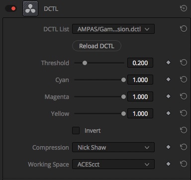
I have made a Resolve DCTL version of @jedsmith’s BlinkScript. This allows it to run in real-time on moving footage.

DCTL_gamut_mapper

5 Likes

That helped me figure it out. Thanks for teaching me math @Thomas_Mansencal :stuck_out_tongue:

I have a few more updates. I figured out the bug with calculating the inverse. It was just a simple thing I missed. I needed to correctly inverse the calculation of the scale factor.

Thanks to Thomas’ help with the tanh function I was able to get the parameters to behave the same between both methods. For the limit controls of cyan, magenta, or yellow: When limit is at 0, no compression is applied. When limit is at 1, out of gamut colors are compressed to the gamut boundary. When limit is greater than 1 (with a max of 1/(1-threshold) which would be a hard clip), out of gamut colors are compressed more than the gamut boundary.

For inverting the gamut compression, there are still differences. I think it is caused by the asymptotic nature of the compression curve and a lack of precision, but it could very well be something else that I’m missing. Anyone sees something I’m not please let me know! :smiley:

I am able to get a perfect roundtrip if I use the original non-gamut compressed image to calculate the achromatic distance from… To allow this workflow I’ve added a “orig” input on the nuke node.

Updated blinkscript and nuke expression node is here:

@nick Thanks for the DCTL! That should be useful. It’s pretty cool how similar CTL and C is, it’s super easy to port C code over.

As before here’s the full source for the blinkscript so it’s easy to look over:

kernel GamutCompression : ImageComputationKernel<ePixelWise> {
  Image<eRead, eAccessPoint, eEdgeClamped> src;
  Image<eWrite> dst;

  param:
    float threshold;
    float cyan;
    float magenta;
    float yellow;
    int method;
    bool invert;
    bool distance;
    bool d_compressed;

  // calc hyperbolic tangent
  float tanh( float in) {
    float e = 2.718281828459f;
    float f = pow(e, 2*in);
    return (f-1.0f) / (f+1.0f);
  }

  // calc inverse hyperbolic tangent
  float atanh( float in) {
    return log((1.0f+in)/(1.0f-in))/2.0f;
  }

  void process() {

    // thr is the complement of threshold. 
    // that is: the percentage of the core gamut to protect
    float thr = 1.0f - threshold;

    // bias limits by color component
    // range is limited to 0.00001 > lim < 1/thr
    // cyan = 0: no compression
    // cyan = 1: "normal" compression with limit at 1.0
    // 1 > cyan < 1/thr : compress more than edge of gamut. max = hard clip (e.g., thr=0.8, max = 1.25)
    float3 lim;
    lim.x = 1.0f/max(0.00001f, min(1.0f/thr, cyan));
    lim.y = 1.0f/max(0.00001f, min(1.0f/thr, magenta));
    lim.z = 1.0f/max(0.00001f, min(1.0f/thr, yellow));

    float r = src().x;
    float g = src().y;
    float b = src().z;

    // achromatic axis 
    float ach = max(r, max(g, b));

    // distance from the achromatic axis for each color component
    float d_r = ach == 0 ? 0 : sqrt( pow(r-ach, 2.0f)) / ach;
    float d_g = ach == 0 ? 0 : sqrt( pow(g-ach, 2.0f)) / ach;
    float d_b = ach == 0 ? 0 : sqrt( pow(b-ach, 2.0f)) / ach;
    

    // compress distance for each color component
    float cd_r, cd_g, cd_b;
    if (method == 0.0f) {
      // hyperbolic tangent softclip method suggested by Thomas Mansencal here
      // https://community.acescentral.com/t/simplistic-gamut-mapping-approaches-in-nuke/2679/2
      // gives good results, but perhaps the curve is too asymptotic. very little color shift.
      // example plot: https://www.desmos.com/calculator/jtvzbae25q
      cd_r = d_r > thr ? thr + (lim.x - thr) * tanh( ( (d_r - thr)/( lim.x-thr))) : d_r;
      cd_g = d_g > thr ? thr + (lim.y - thr) * tanh( ( (d_g - thr)/( lim.y-thr))) : d_g;
      cd_b = d_b > thr ? thr + (lim.z - thr) * tanh( ( (d_b - thr)/( lim.z-thr))) : d_b;

      if (invert == 1.0f) {
          cd_r = d_r > thr ? thr + (lim.x - thr) * atanh( d_r/( lim.x - thr) - thr/( lim.x - thr)) : d_r;
          cd_g = d_g > thr ? thr + (lim.y - thr) * atanh( d_g/( lim.y - thr) - thr/( lim.y - thr)) : d_g;
          cd_b = d_b > thr ? thr + (lim.z - thr) * atanh( d_b/( lim.z - thr) - thr/( lim.z - thr)) : d_b;
      }
    } else if (method == 1.0f) {
      // softclip method suggested by Nick Shaw here
      // https://community.acescentral.com/t/simplistic-gamut-mapping-approaches-in-nuke/2679/3
      // good results, easy to bias look with limits
      // example plot: https://www.desmos.com/calculator/jyewfptd4y
      cd_r = d_r > thr ? thr+(-1/((d_r-thr)/(lim.x-thr)+1)+1)*(lim.x-thr) : d_r;
      cd_g = d_g > thr ? thr+(-1/((d_g-thr)/(lim.y-thr)+1)+1)*(lim.y-thr) : d_g;
      cd_b = d_b > thr ? thr+(-1/((d_b-thr)/(lim.z-thr)+1)+1)*(lim.z-thr) : d_b;

      if (invert == 1.0f) {
        // inversed compression distance for each color component
        cd_r = d_r > thr ? (pow(thr, 2.0f) - thr*d_r + (lim.x-thr)*d_r) / (thr + (lim.x-thr) - d_r) : d_r;
        cd_g = d_g > thr ? (pow(thr, 2.0f) - thr*d_g + (lim.y-thr)*d_g) / (thr + (lim.y-thr) - d_g) : d_g;
        cd_b = d_b > thr ? (pow(thr, 2.0f) - thr*d_b + (lim.z-thr)*d_b) / (thr + (lim.z-thr) - d_b) : d_b;
      }
    }

    float c_r, c_g, c_b;
    if (invert == 1.0f) {
      // scale up each color component relative to achromatic axis by gamut uncompression factor
      c_r = (r-ach)*((cd_r-d_r)+1.0f)+ach;
      c_g = (g-ach)*((cd_g-d_g)+1.0f)+ach;
      c_b = (b-ach)*((cd_b-d_b)+1.0f)+ach;

    } else {
      // scale down each color component relative to achromatic axis by gamut compression factor
      c_r = (r-ach)/((d_r-cd_r)+1.0f)+ach;
      c_g = (g-ach)/((d_g-cd_g)+1.0f)+ach;
      c_b = (b-ach)/((d_b-cd_b)+1.0f)+ach;
    }

    // write to output
    dst() = float4(c_r, c_g, c_b, 1);

    // debug outputs
    if (distance == 1.0f) {
      if (d_compressed == 1.0f) {
        dst() = float4(cd_r, cd_g, cd_b, 1.0f);
      } else {
        dst() = float4(d_r, d_g, d_b, 1.0f);
      }
    }
  }
};
2 Likes

That works very well! Better out-of-the-box than everything I have been musing with so far (I get very similar output by tweaking parameterisation but not as a default), really like how simple and elegant this is. :smiling_face_with_three_hearts:

Cheers,

Thomas

2 Likes

Yeah Jed, this is great work! Will message you about talking through some of the details at a future meeting soon.

Ran Jed’s Model through the two images I’m using currently to do my tests:

Jed’s RGB Saturation Based Model - Threshold 0.15

Thomas’s HSV Control Based Model - Threshold & Hue Twist Controls Tweaked

Thomas’s HSV Control Based Model - Threshold 0.15
Note that with default parameters, the model is almost the same than the HSV model of @matthias.scharfenber.

I can get close to Jed’s with mine using the Hue Twists and fiddling a bit with the Threshold but Jed’s default to a much more pleasing output, i.e. less magenta, the Model is simpler, more elegant, faster and easier to implement.

Cheers,

Thomas

The magenta feels like the other half of the missing gamut map, no? Any idea on whether the values are escaping the gamut volume there?

I had planned to update my DCTL implementation to match @jedsmith’s latest BlinkScript. But he has very kindly already done that in his own fork, and submitted a pull request, which I have just merged. Everybody who is testing it should grab the latest version.

2 Likes

from my experience, Jed’s method (I will call it Kirk method :slight_smile: ) works good for scene-referred data for a general any gamut to any gamut mapper, and it ticks all the boxes we have defined :-).

2 Likes

@daniele: I wanted to ask you how close it is from the Filmlight one, seemed quite similar in principle to what you presented a few weeks ago.

It is a pretty similar approach, yes.

1 Like

I was playing around with different tone-mapping algorithms to use for compression of the distance, and came up with a new one based on a natural exponent function. It is between the hyperbolic tangent function and the Reinhard style simple tone-mapping function in terms of the aggressiveness of its slope. I think the results are pretty good.

Here’s a plot comparing all three compression functions: https://www.desmos.com/calculator/x69iyptspq

And here’s a few screenshots comparing the three methods


As before, here are the

and source code

kernel GamutCompression : ImageComputationKernel<ePixelWise> {
  Image<eRead, eAccessPoint, eEdgeClamped> src;
  Image<eWrite> dst;

  param:
    float threshold;
    float cyan;
    float magenta;
    float yellow;
    int method;
    bool invert;
    bool distance;
    bool d_compressed;

  // calc hyperbolic tangent
  float tanh( float in) {
    float e = 2.718281828459f;
    float f = pow(e, 2*in);
    return (f-1.0f) / (f+1.0f);
  }

  // calc inverse hyperbolic tangent
  float atanh( float in) {
    return log((1.0f+in)/(1.0f-in))/2.0f;
  }

  void process() {

    // thr is the complement of threshold. 
    // that is: the percentage of the core gamut to protect
    float thr = 1.0f - threshold;

    // bias limits by color component
    // range is limited to 0.00001 > lim < 1/thr
    // cyan = 0: no compression
    // cyan = 1: "normal" compression with limit at 1.0
    // 1 > cyan < 1/thr : compress more than edge of gamut. max = hard clip (e.g., thr=0.8, max = 1.25)
    float3 lim;
    lim.x = 1.0f/max(0.00001f, min(1.0f/thr, cyan));
    lim.y = 1.0f/max(0.00001f, min(1.0f/thr, magenta));
    lim.z = 1.0f/max(0.00001f, min(1.0f/thr, yellow));

    float r = src().x;
    float g = src().y;
    float b = src().z;

    // achromatic axis 
    float ach = max(r, max(g, b));

    // distance from the achromatic axis for each color component
    float d_r = ach == 0 ? 0 : sqrt( pow(r-ach, 2.0f)) / ach;
    float d_g = ach == 0 ? 0 : sqrt( pow(g-ach, 2.0f)) / ach;
    float d_b = ach == 0 ? 0 : sqrt( pow(b-ach, 2.0f)) / ach;
    

    // compress distance for each color component
    float cd_r, cd_g, cd_b;
    if (method == 0.0f) {
      // hyperbolic tangent softclip method suggested by Thomas Mansencal here
      // https://community.acescentral.com/t/simplistic-gamut-mapping-approaches-in-nuke/2679/2
      // gives good results, but perhaps the curve is too asymptotic. very little color shift.
      // example plot: https://www.desmos.com/calculator/jtvzbae25q
      cd_r = d_r > thr ? thr + (lim.x - thr) * tanh( ( (d_r - thr)/( lim.x-thr))) : d_r;
      cd_g = d_g > thr ? thr + (lim.y - thr) * tanh( ( (d_g - thr)/( lim.y-thr))) : d_g;
      cd_b = d_b > thr ? thr + (lim.z - thr) * tanh( ( (d_b - thr)/( lim.z-thr))) : d_b;

      if (invert == 1.0f) {
          cd_r = d_r > thr ? thr + (lim.x - thr) * atanh( d_r/( lim.x - thr) - thr/( lim.x - thr)) : d_r;
          cd_g = d_g > thr ? thr + (lim.y - thr) * atanh( d_g/( lim.y - thr) - thr/( lim.y - thr)) : d_g;
          cd_b = d_b > thr ? thr + (lim.z - thr) * atanh( d_b/( lim.z - thr) - thr/( lim.z - thr)) : d_b;
      }
    } else if (method == 1.0f) {
      // softclip method suggested by Nick Shaw here
      // https://community.acescentral.com/t/simplistic-gamut-mapping-approaches-in-nuke/2679/3
      // good results, easy to bias look with limits
      // example plot: https://www.desmos.com/calculator/jyewfptd4y
      cd_r = d_r > thr ? thr+(-1/((d_r-thr)/(lim.x-thr)+1)+1)*(lim.x-thr) : d_r;
      cd_g = d_g > thr ? thr+(-1/((d_g-thr)/(lim.y-thr)+1)+1)*(lim.y-thr) : d_g;
      cd_b = d_b > thr ? thr+(-1/((d_b-thr)/(lim.z-thr)+1)+1)*(lim.z-thr) : d_b;

      if (invert == 1.0f) {
        // inversed compression distance for each color component
        cd_r = d_r > thr ? (pow(thr, 2.0f) - thr*d_r + (lim.x-thr)*d_r) / (thr + (lim.x-thr) - d_r) : d_r;
        cd_g = d_g > thr ? (pow(thr, 2.0f) - thr*d_g + (lim.y-thr)*d_g) / (thr + (lim.y-thr) - d_g) : d_g;
        cd_b = d_b > thr ? (pow(thr, 2.0f) - thr*d_b + (lim.z-thr)*d_b) / (thr + (lim.z-thr) - d_b) : d_b;
      }
    }

    float c_r, c_g, c_b;
    if (invert == 1.0f) {
      // scale up each color component relative to achromatic axis by gamut uncompression factor
      c_r = (r-ach)*((cd_r-d_r)+1.0f)+ach;
      c_g = (g-ach)*((cd_g-d_g)+1.0f)+ach;
      c_b = (b-ach)*((cd_b-d_b)+1.0f)+ach;

    } else {
      // scale down each color component relative to achromatic axis by gamut compression factor
      c_r = (r-ach)/((d_r-cd_r)+1.0f)+ach;
      c_g = (g-ach)/((d_g-cd_g)+1.0f)+ach;
      c_b = (b-ach)/((d_b-cd_b)+1.0f)+ach;
    }

    // write to output
    dst() = float4(c_r, c_g, c_b, 1);

    // debug outputs
    if (distance == 1.0f) {
      if (d_compressed == 1.0f) {
        dst() = float4(cd_r, cd_g, cd_b, 1.0f);
      } else {
        dst() = float4(d_r, d_g, d_b, 1.0f);
      }
    }
  }
};
2 Likes

Hi @jedsmith,

Something you will find is that the derivatives of all those functions (besides tanh) are not smooth which means that there is a kink at the graft point, it is probably not visible but it is important to be aware of. I added them to your Desmos example: https://www.desmos.com/calculator/bt901oznbm

Cheers,

Thomas

PS: This goes without saying that I favour smooth derivatives! :slight_smile:

Curious what specific portion of the chain is causing this posterization error:

@Troy_James_Sobotka it looks like this is caused by brightening of the out of gamut areas of the face, which have less noise from the camera sensor. I made a little screencapture and uploaded it in a terribly compressed gif with lots of posterization … hopefully it gets the idea across anyway :stuck_out_tongue:

This one is with the tanh curve
face_gamut_compress_tanh

This one is with the “simple” curve.
face_gamut_compress_simple

Interestingly, the “simple” compression method with a limit of around 0.8 has less of this visual artifact.

With the much more aggressive slope of the “simple” curve and limiting it to 0.8, it brings the question: how far outside of gamut do we need to go when compressing values in? And if it’s not to infinity, what compression curve has the least visual artifacts? This is something I think we need to figure out.

1 Like

Another update:
I have fixed the invertibility issues.

I realized after an embarrassingly long time that c_r could be defined completely in terms of ach and cd_r (achromatic and compressed distance, respectively). This allows the gamut compression to be exactly inverted.

As before:

kernel GamutCompression : ImageComputationKernel<ePixelWise> {
  Image<eRead, eAccessPoint, eEdgeClamped> src;
  Image<eWrite> dst;

  param:
    float threshold;
    float cyan;
    float magenta;
    float yellow;
    int method;
    bool invert;

  // calc hyperbolic tangent
  float tanh( float in) {
    float f = exp(2.0f*in);
    return (f-1.0f) / (f+1.0f);
  }

  // calc inverse hyperbolic tangent
  float atanh( float in) {
    return log((1.0f+in)/(1.0f-in))/2.0f;
  }

  void process() {
    // thr is the complement of threshold. 
    // that is: the percentage of the core gamut to protect
    float thr = 1.0f - threshold;

    // bias limits by color component
    // range is limited to 0.00001 > lim < 1/thr
    // cyan = 0: no compression
    // cyan = 1: "normal" compression with limit at 1.0
    // 1 > cyan < 1/thr : compress more than edge of gamut. max = hard clip (e.g., thr=0.8, max = 1.25)
    float3 lim;
    lim.x = 1.0f/max(0.00001f, min(1.0f/thr, cyan));
    lim.y = 1.0f/max(0.00001f, min(1.0f/thr, magenta));
    lim.z = 1.0f/max(0.00001f, min(1.0f/thr, yellow));

    float r = src().x;
    float g = src().y;
    float b = src().z;

    // achromatic axis 
    float ach = max(r, max(g, b));

    // distance from the achromatic axis for each color component
    float d_r, d_g, d_b;
    d_r = ach == 0 ? 0 : fabs(float(r-ach)) / ach;
    d_g = ach == 0 ? 0 : fabs(float(g-ach)) / ach;
    d_b = ach == 0 ? 0 : fabs(float(b-ach)) / ach;

    // compress distance for each color component
    // method 0 : tanh - hyperbolic tangent compression method suggested by Thomas Mansencal https://community.acescentral.com/t/simplistic-gamut-mapping-approaches-in-nuke/2679/2
    // method 1 : exp - natural exponent compression method
    // method 2 : simple - simple Reinhard type compression suggested by Nick Shaw https://community.acescentral.com/t/simplistic-gamut-mapping-approaches-in-nuke/2679/3
    // example plots for each method: https://www.desmos.com/calculator/x69iyptspq
    float cd_r, cd_g, cd_b;
    if (method == 0.0f) {
      if (invert == 0.0f) {
        cd_r = d_r > thr ? thr + (lim.x - thr) * tanh( ( (d_r - thr)/( lim.x-thr))) : d_r;
        cd_g = d_g > thr ? thr + (lim.y - thr) * tanh( ( (d_g - thr)/( lim.y-thr))) : d_g;
        cd_b = d_b > thr ? thr + (lim.z - thr) * tanh( ( (d_b - thr)/( lim.z-thr))) : d_b;
      } else {
          cd_r = d_r > thr ? thr + (lim.x - thr) * atanh( d_r/( lim.x - thr) - thr/( lim.x - thr)) : d_r;
          cd_g = d_g > thr ? thr + (lim.y - thr) * atanh( d_g/( lim.y - thr) - thr/( lim.y - thr)) : d_g;
          cd_b = d_b > thr ? thr + (lim.z - thr) * atanh( d_b/( lim.z - thr) - thr/( lim.z - thr)) : d_b;
      }
    } else if (method == 1.0f) {
      if (invert == 0.0f) {
        cd_r = d_r > thr ? lim.x-(lim.x-thr)*exp(-(((d_r-thr)*((1.0f*lim.x)/(lim.x-thr))/lim.x))) : d_r;
        cd_g = d_g > thr ? lim.y-(lim.y-thr)*exp(-(((d_g-thr)*((1.0f*lim.y)/(lim.y-thr))/lim.y))) : d_g;
        cd_b = d_b > thr ? lim.z-(lim.z-thr)*exp(-(((d_b-thr)*((1.0f*lim.z)/(lim.z-thr))/lim.z))) : d_b;
      } else {
        cd_r = d_r > thr ? -log( (d_r-lim.x)/(thr-lim.x))*(-thr+lim.x)/1.0f+thr : d_r;
        cd_g = d_g > thr ? -log( (d_g-lim.y)/(thr-lim.y))*(-thr+lim.y)/1.0f+thr : d_g;
        cd_b = d_b > thr ? -log( (d_b-lim.z)/(thr-lim.z))*(-thr+lim.z)/1.0f+thr : d_b;
      }
    } else if (method == 2.0f) {
      if (invert == 0.0f) {
        cd_r = d_r > thr ? thr+(-1/((d_r-thr)/(lim.x-thr)+1)+1)*(lim.x-thr) : d_r;
        cd_g = d_g > thr ? thr+(-1/((d_g-thr)/(lim.y-thr)+1)+1)*(lim.y-thr) : d_g;
        cd_b = d_b > thr ? thr+(-1/((d_b-thr)/(lim.z-thr)+1)+1)*(lim.z-thr) : d_b;
      } else {
        cd_r = d_r > thr ? (pow(thr, 2.0f) - thr*d_r + (lim.x-thr)*d_r) / (thr + (lim.x-thr) - d_r) : d_r;
        cd_g = d_g > thr ? (pow(thr, 2.0f) - thr*d_g + (lim.y-thr)*d_g) / (thr + (lim.y-thr) - d_g) : d_g;
        cd_b = d_b > thr ? (pow(thr, 2.0f) - thr*d_b + (lim.z-thr)*d_b) / (thr + (lim.z-thr) - d_b) : d_b;
      }
    }

    // scale each color component relative to achromatic axis by gamut compression factor
    float c_r, c_g, c_b;
    c_r = ach-cd_r*ach;
    c_g = ach-cd_g*ach;
    c_b = ach-cd_b*ach;

    // write to output
    dst() = float4(c_r, c_g, c_b, 1);

  }
};