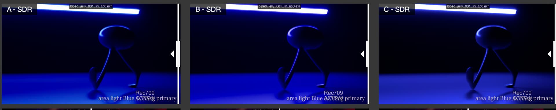
A sampling of how blue is looking in candidates A,B, and C in SDR
Image 20.exr (20.avif):
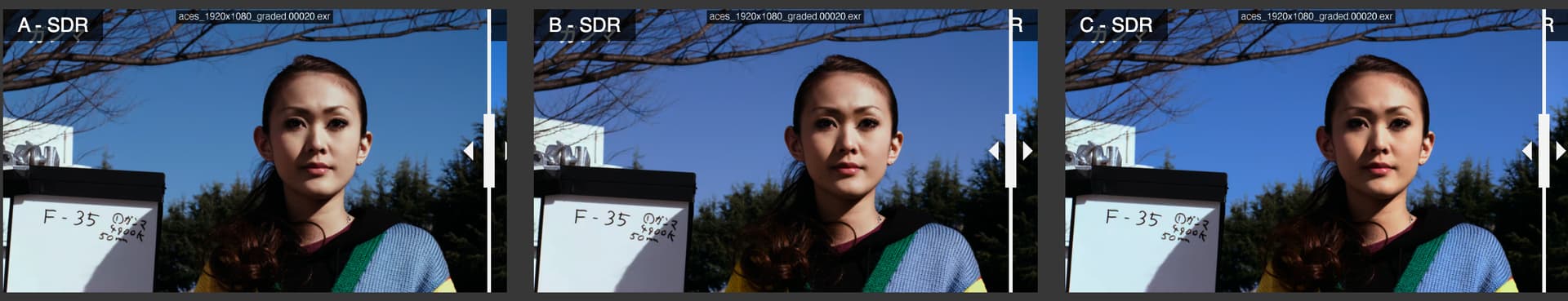
image 295.exr (179.avif):
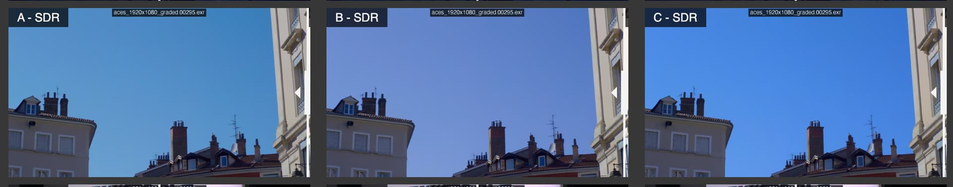
image 358.exr (239.avif):
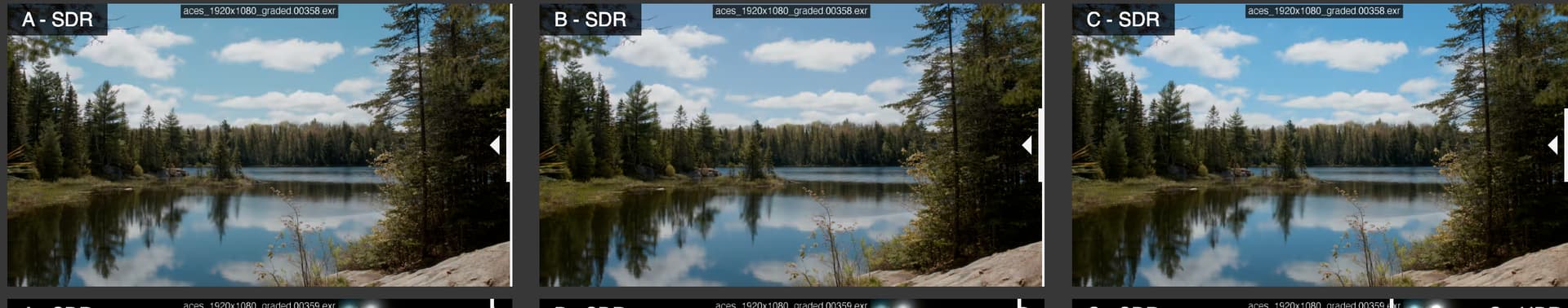
image 342.er (223.avif):
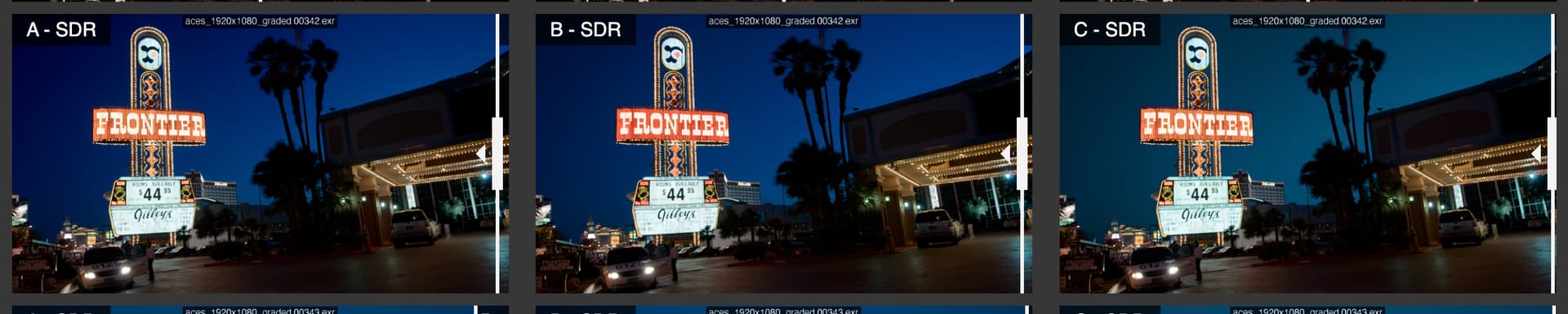
image 562.exr (437.avif)
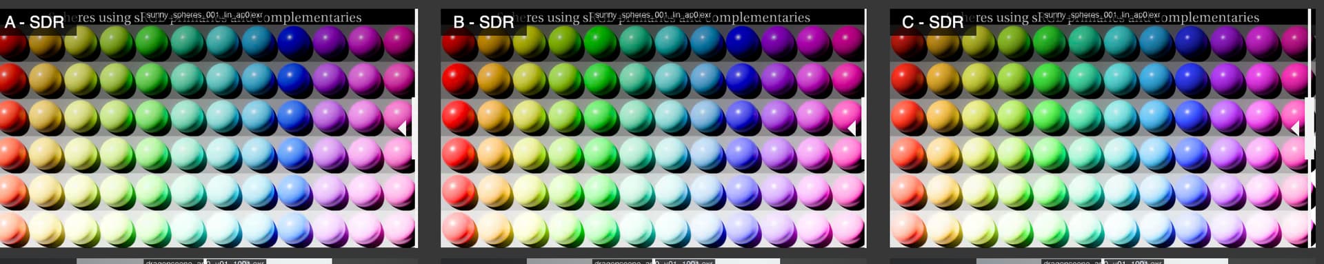
image 562.exr (482.avif):
A sampling of how blue is looking in candidates A,B, and C in SDR
Image 20.exr (20.avif):
image 295.exr (179.avif):
image 358.exr (239.avif):
image 342.er (223.avif):
image 562.exr (437.avif)
image 562.exr (482.avif):
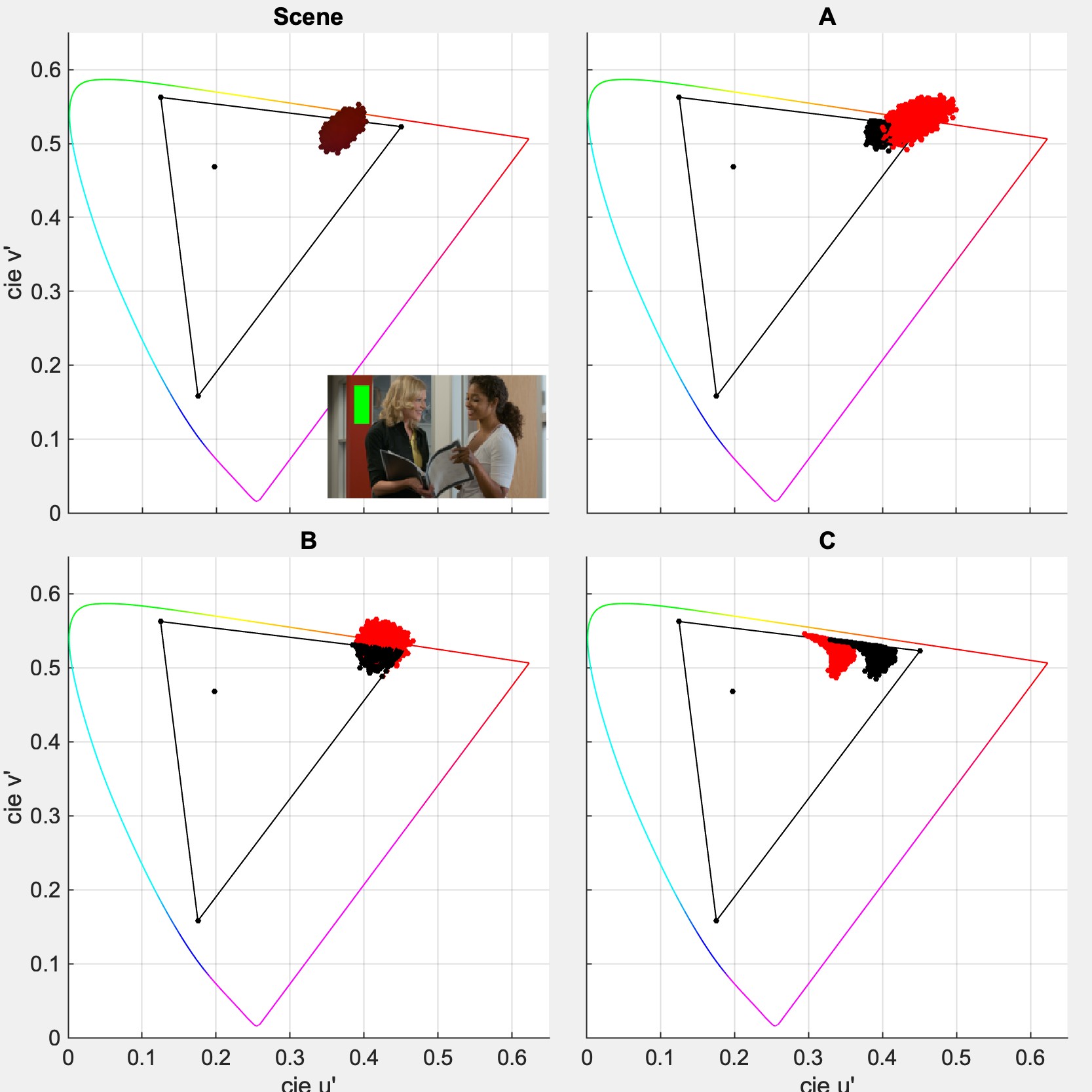
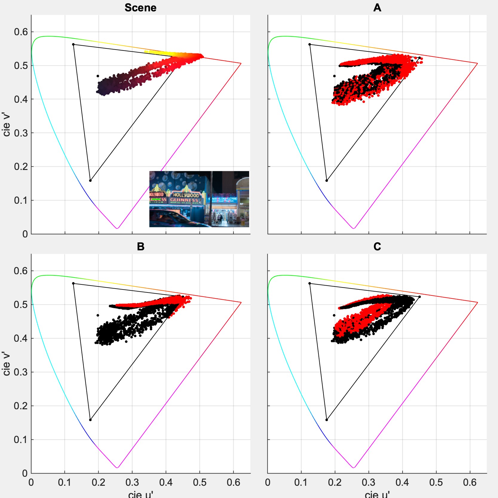
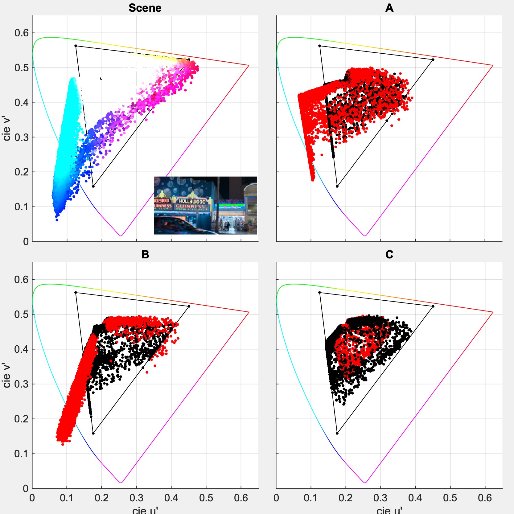
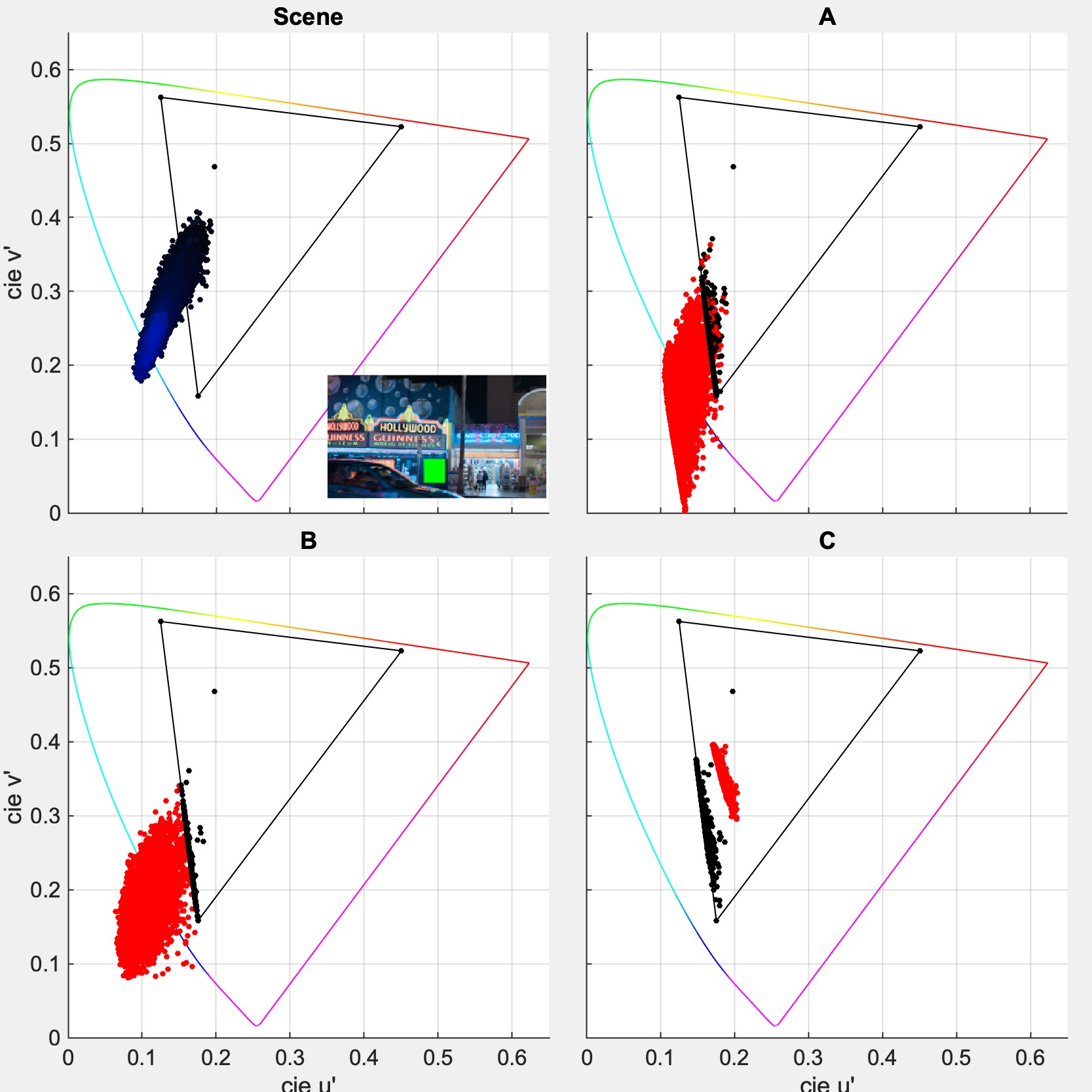
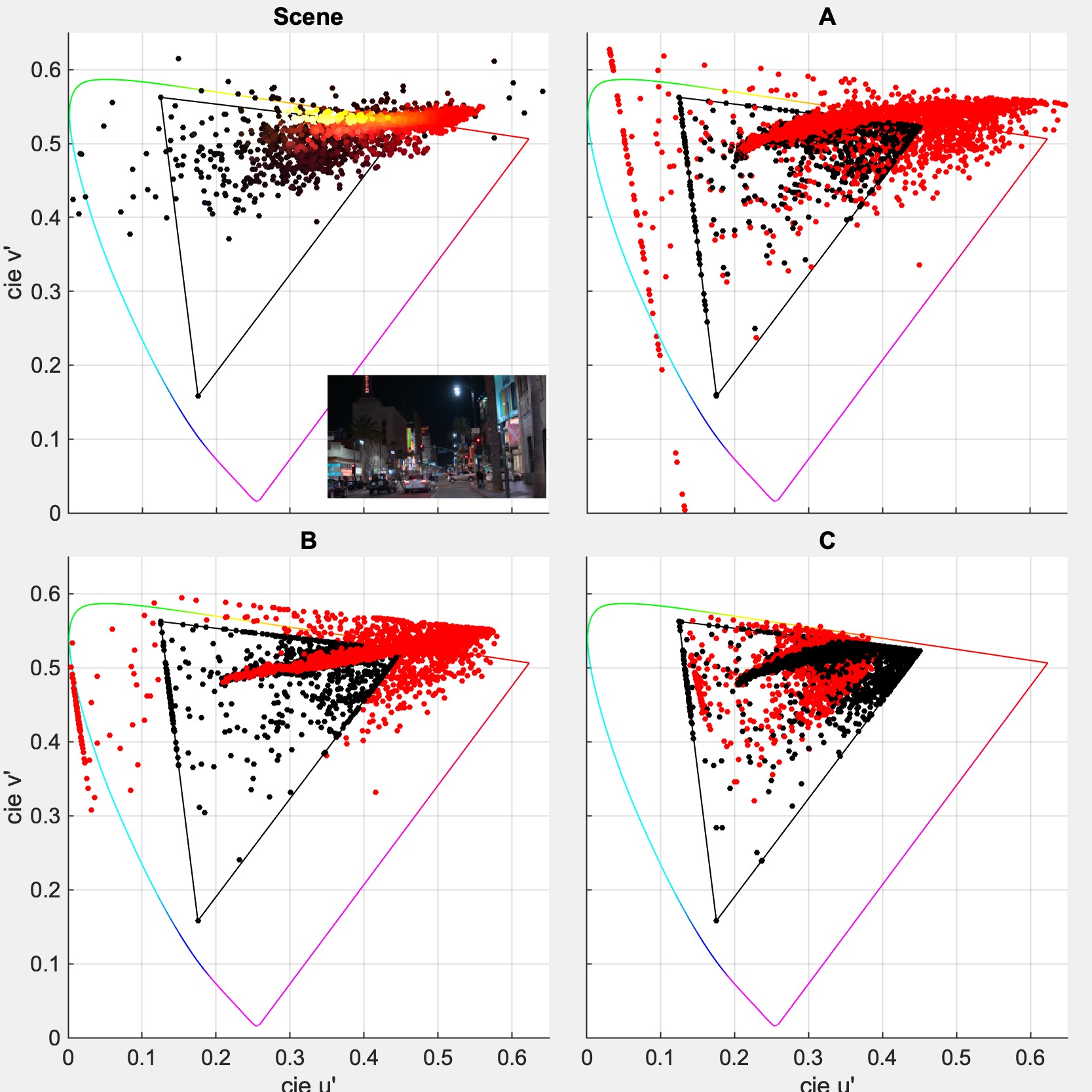
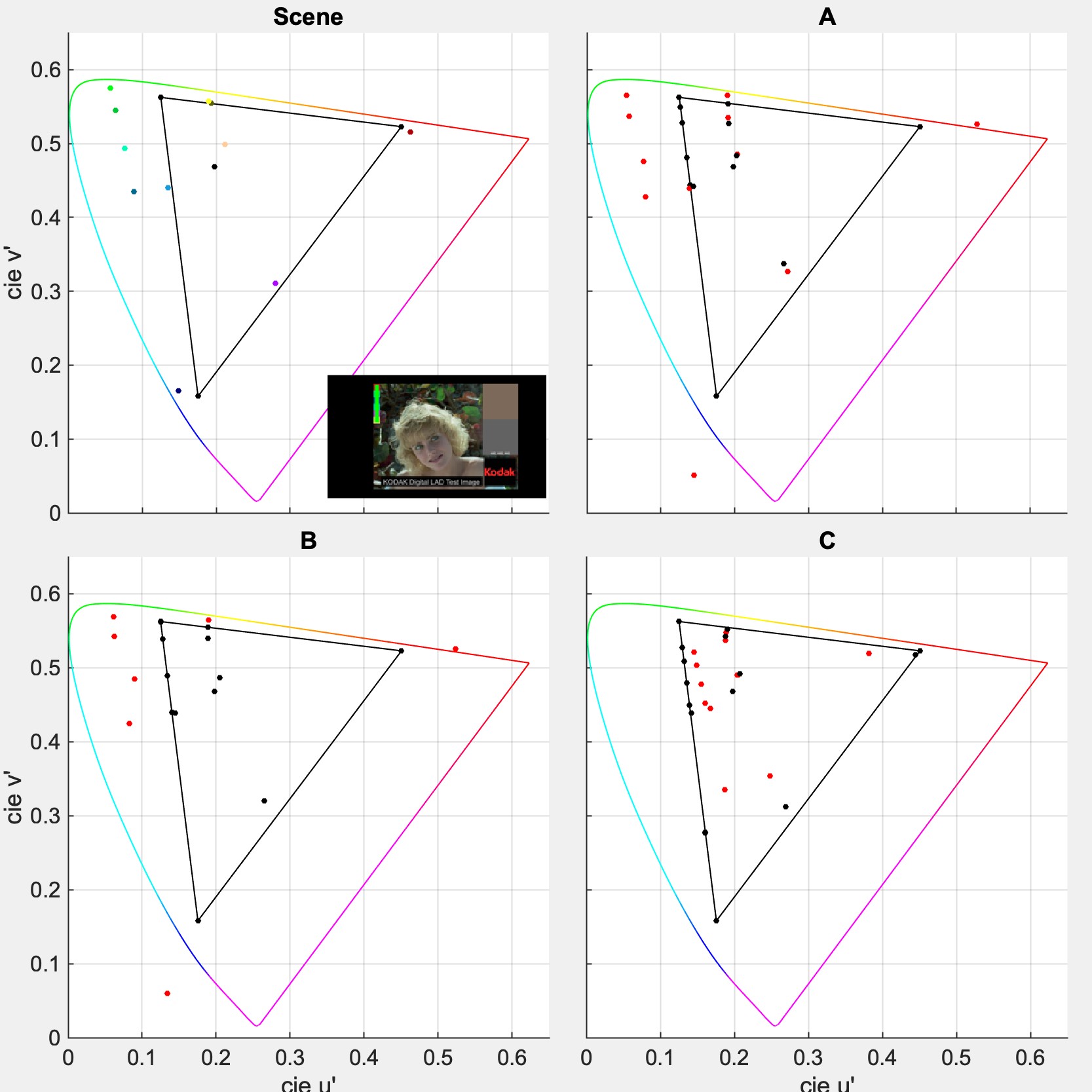
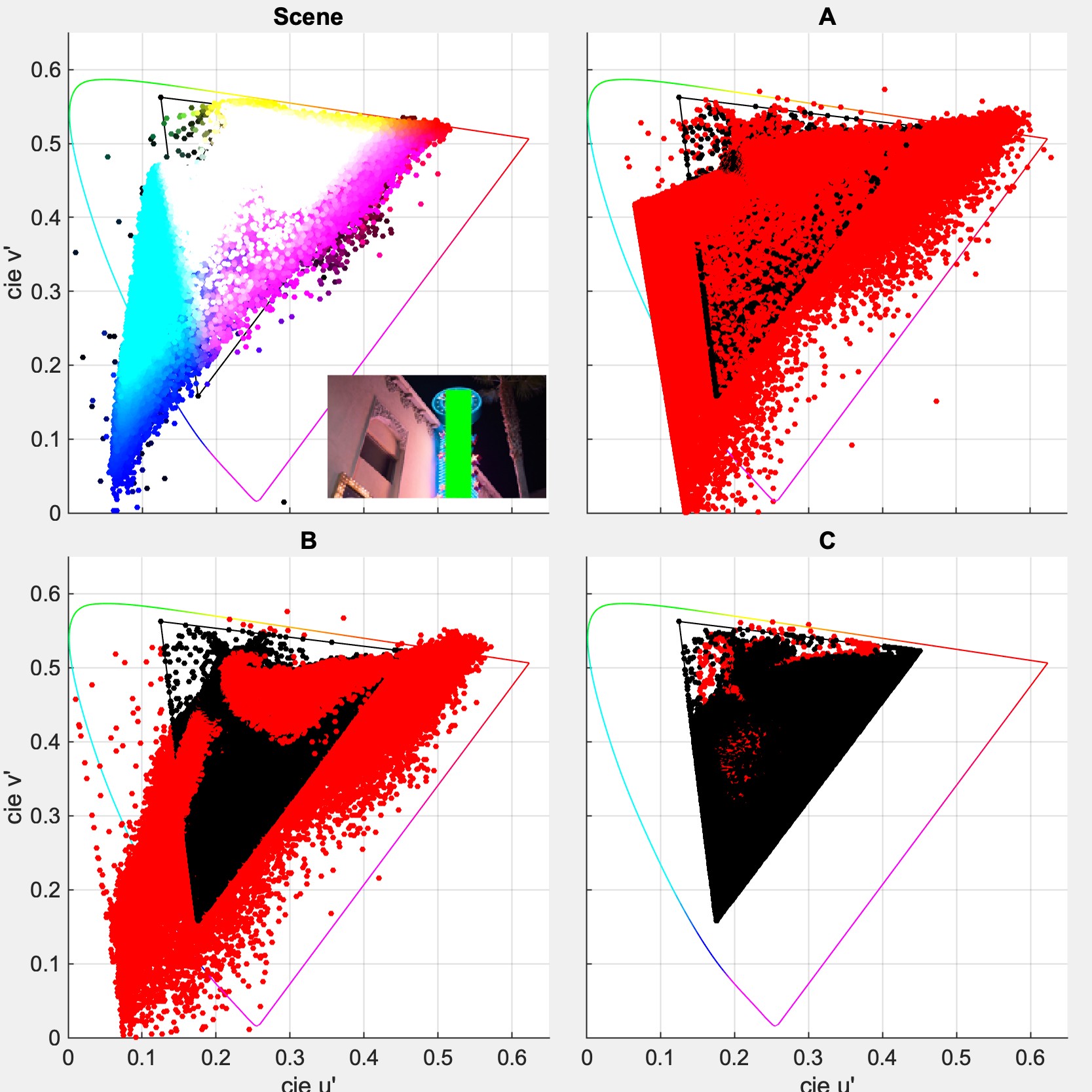
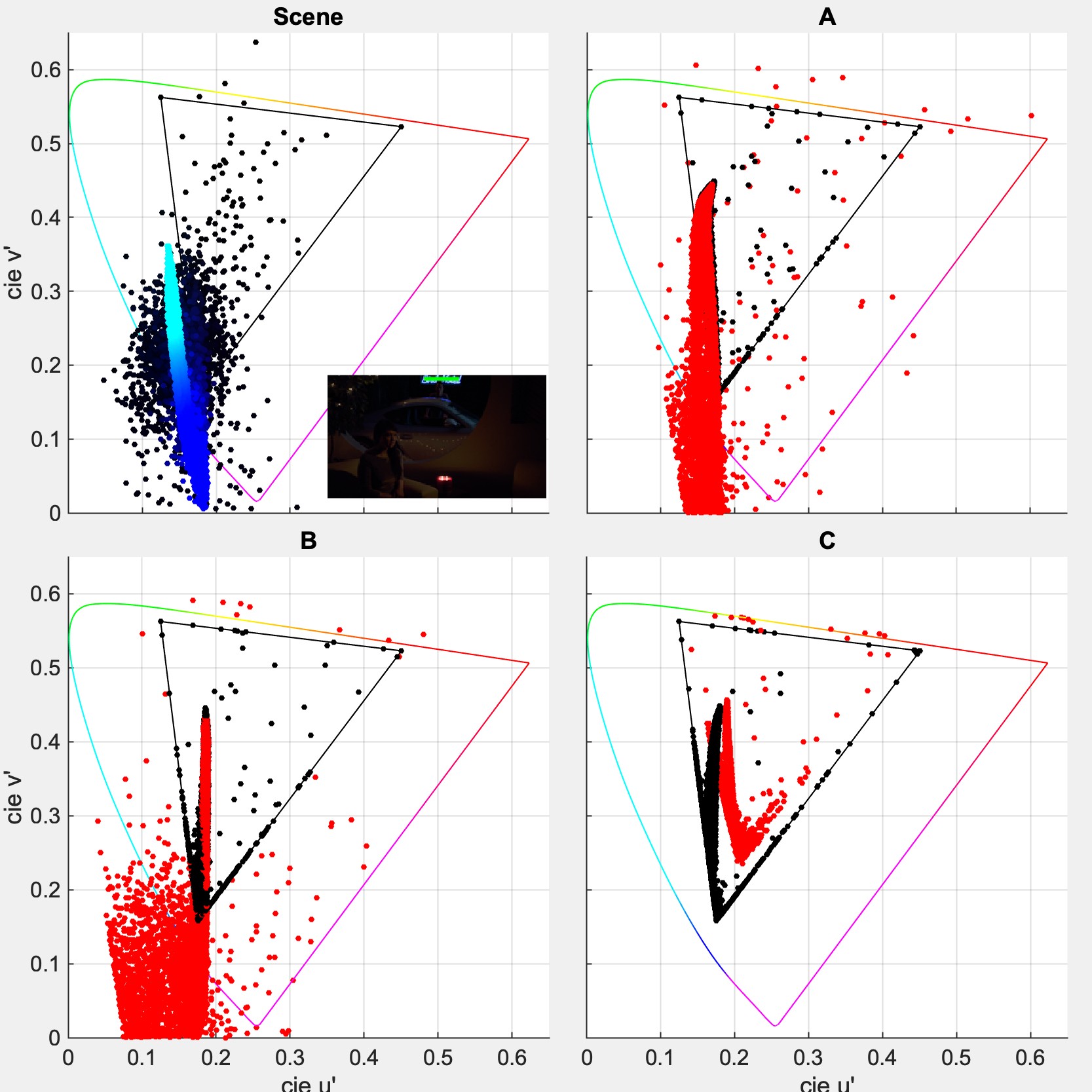
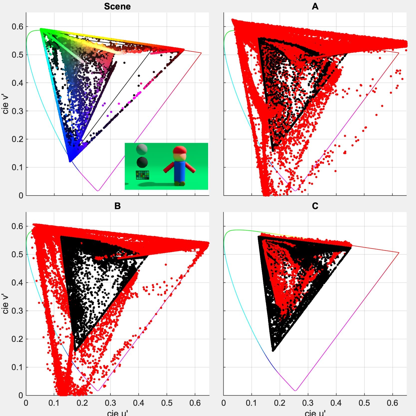
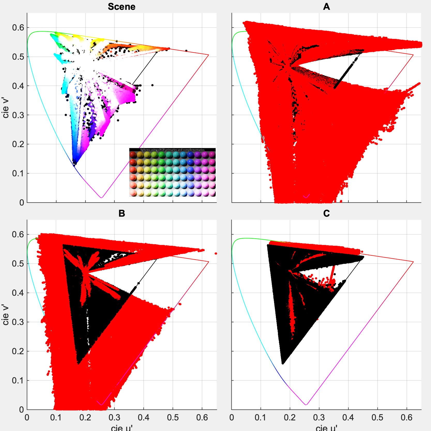
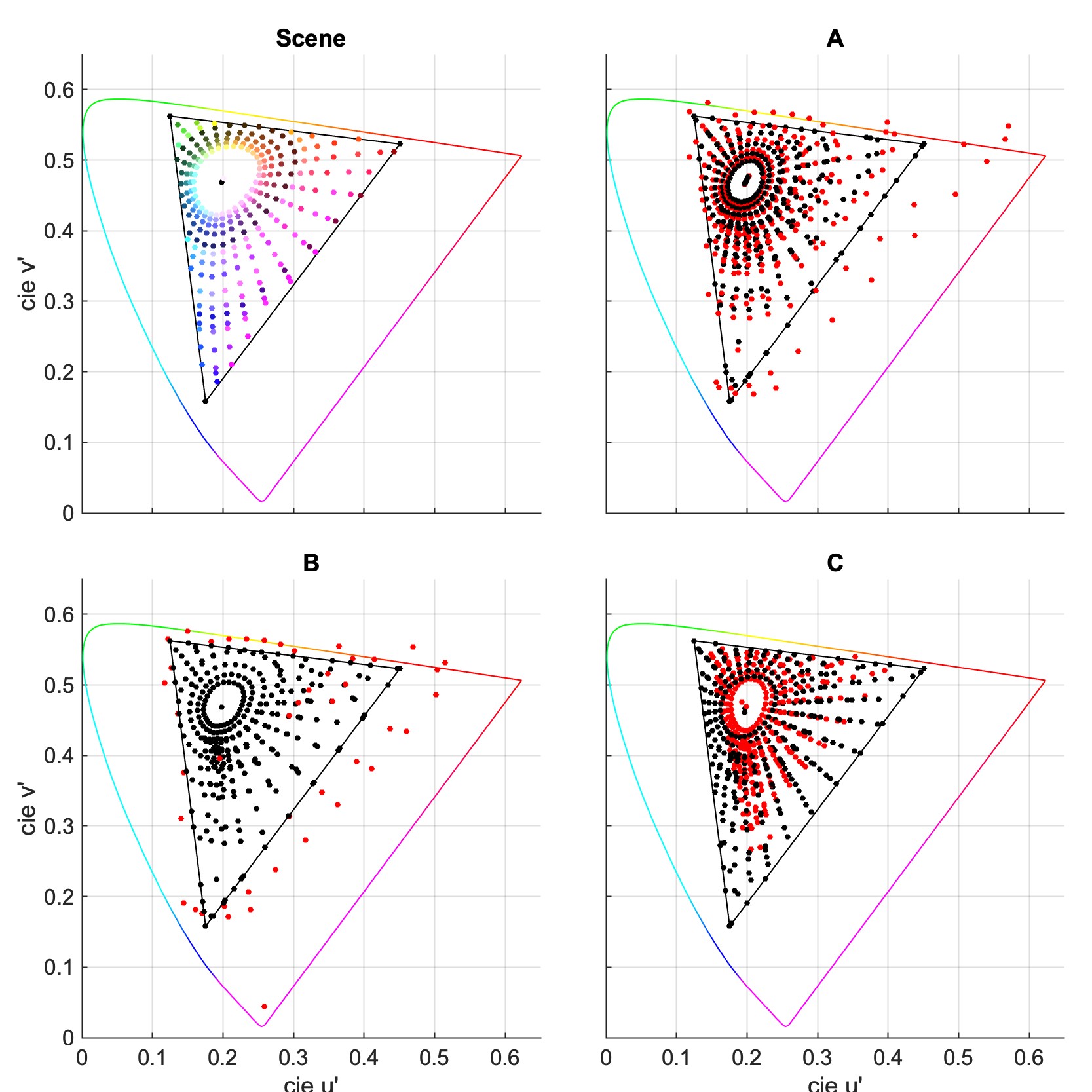
Hard to say what I’m supposed to be looking at without the source images and, for bonus points, chromaticity plots in xyY space since I’m not familiar with all of those source images… What I do know though is that those results are consistent with the algorithms of each candidate. Candidate A which I now know is based on rgbDT has a correction in perceptual space that mostly affects blues and reds. Candidate B doesn’t do anything special for blues so you end up with them moving towards purple as they desaturate because of Abney effect. Candidate C (ZCAMish DRT) does complex gamut mapping in JMh space and sometimes get them right, sometimes get them wrong. As can be noticed on the night scene, it’s worse on very deep dark blues, i.e. I never saw a cyanish night sky in real life.
These are from the cool new SDR/HDR webpage @alexfry posted.
https://alexfry.github.io/ACES_ODT_Candidates_Examples/
I’d also be interested in the sources to these images. There’s lots of great stuff in there! A lot are, I believe, are from @sdyer. I think these were posted on aces central, but I’m not quite sure where. Hopefully someone else can share the link.
I am working on some graphs illustrating where the these blues (and some reds) start out in scene colorimetry, where they end up after the rendering, and where they end up after clipping to display.
(I have some other projects to support first before I’ll have time to get to this but I’ll upload some analysis soon.)
Ask and thou shall receive!
Alex updated all the images with burned in plots:
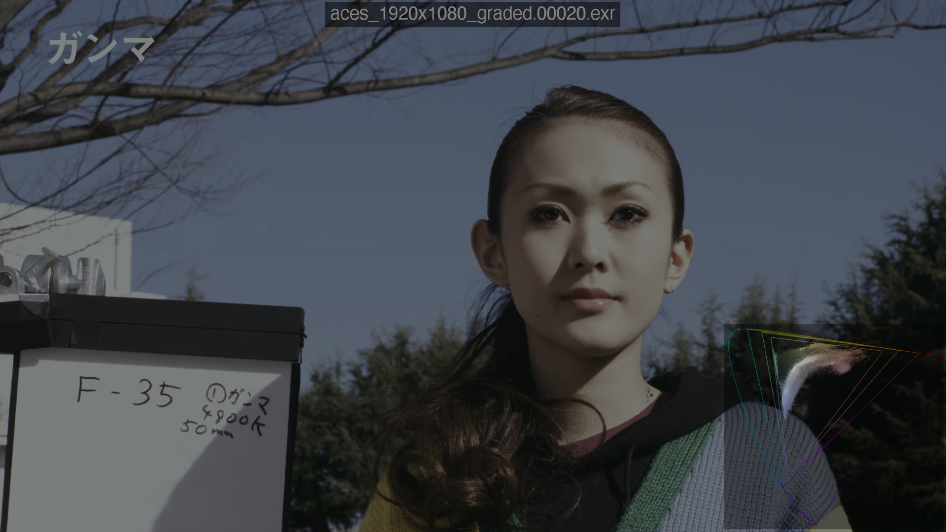
I’ll label the images above with their numbers. For example the first image is #20
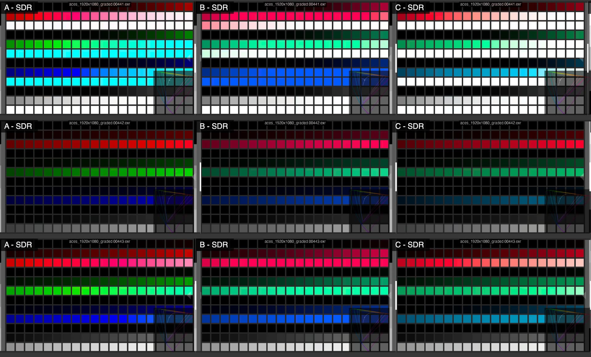
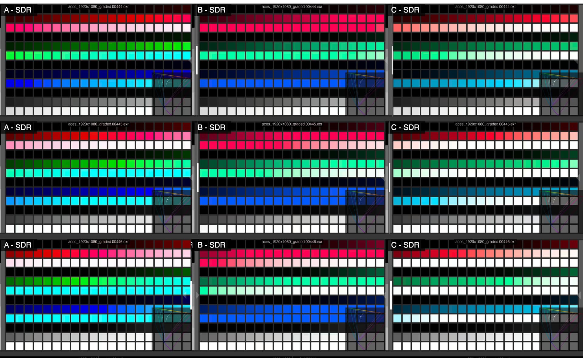
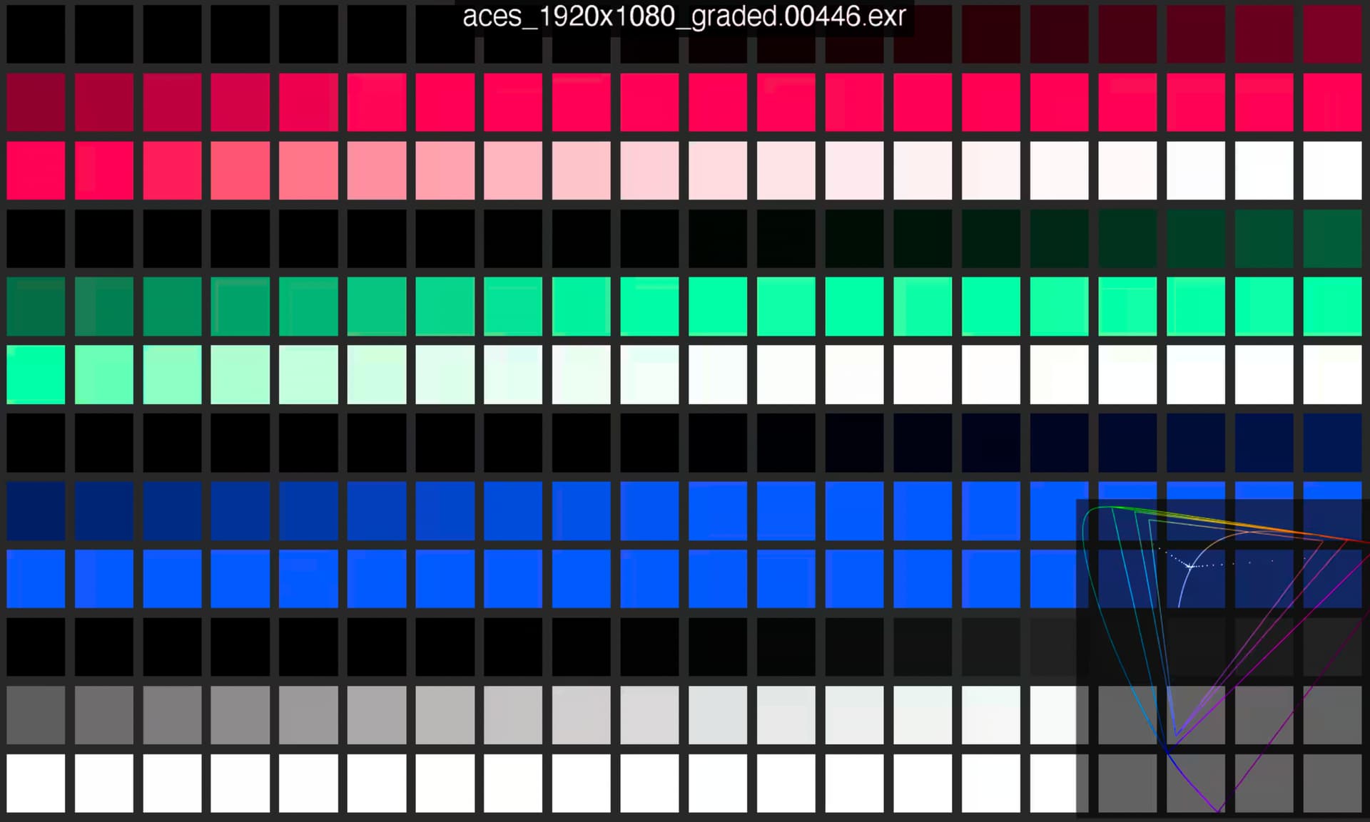
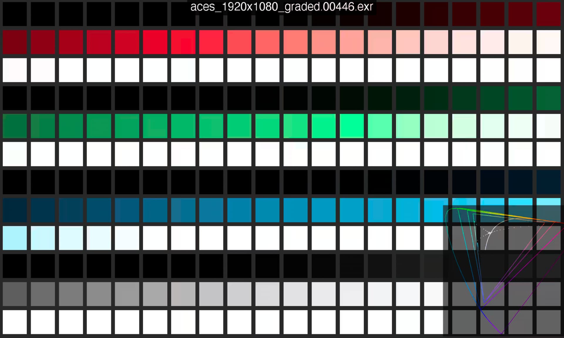
Also these exposure sweeps of are worth noting: (440-446 exr / 316-322.avif)
322.avif SDR Candidate A:
322.avif SDR Candidate B:
322.avif SDR Candidate C:
Added some new features to the comparison pages.
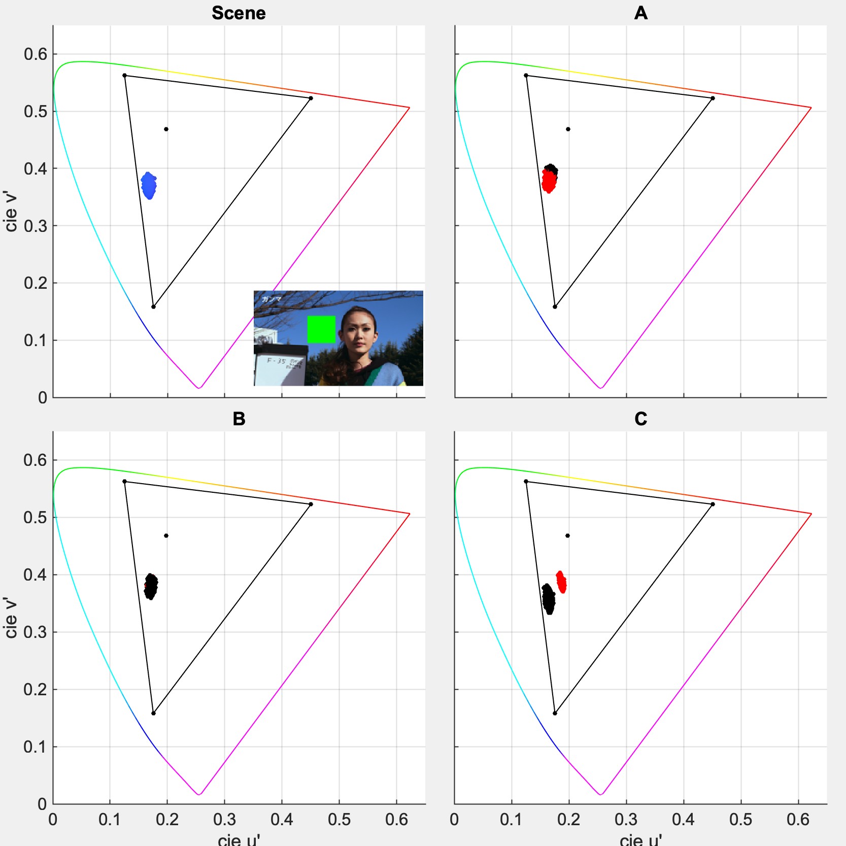
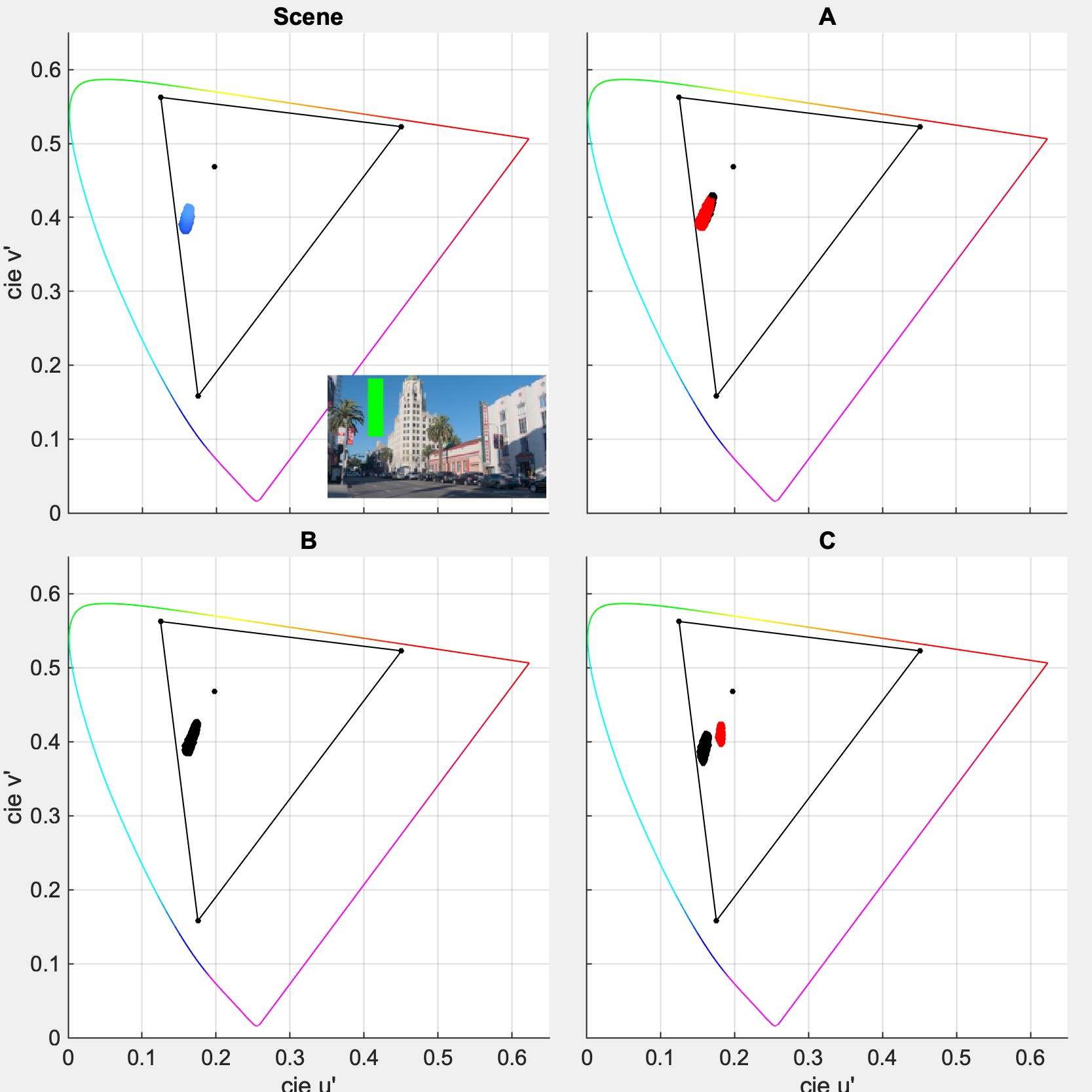
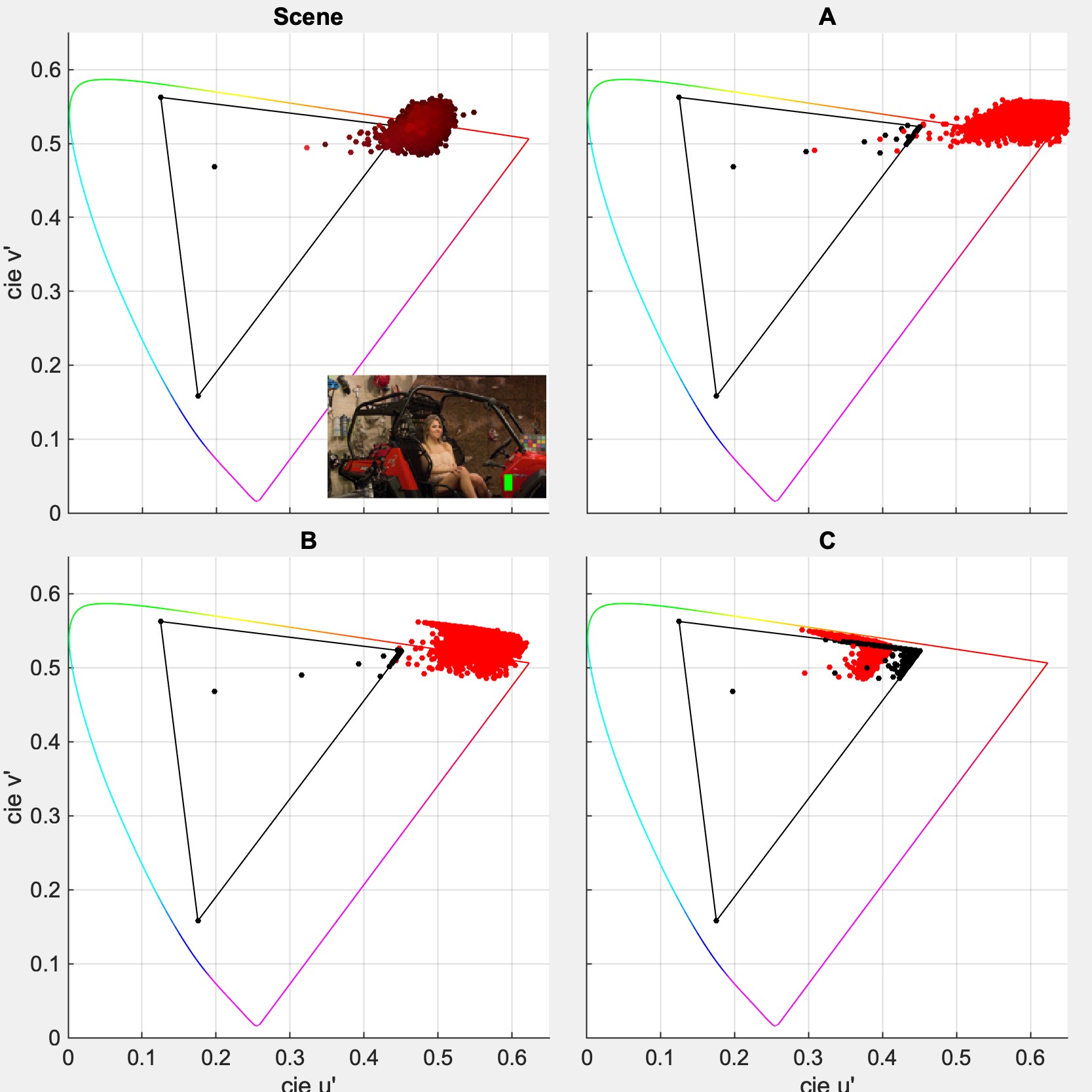
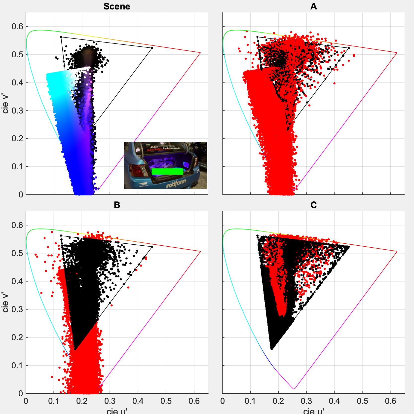
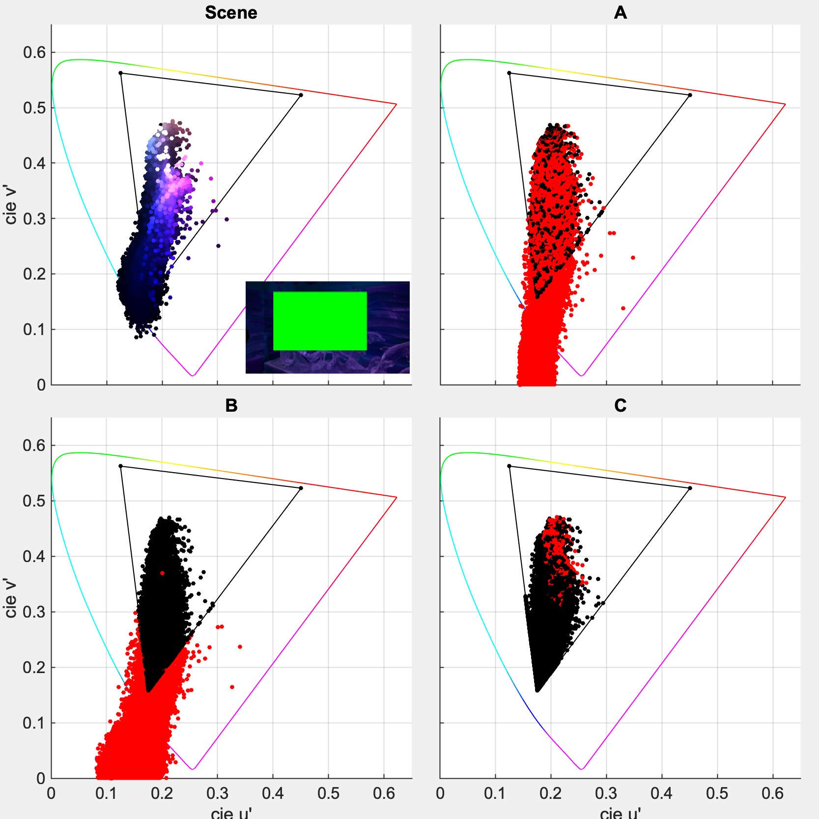
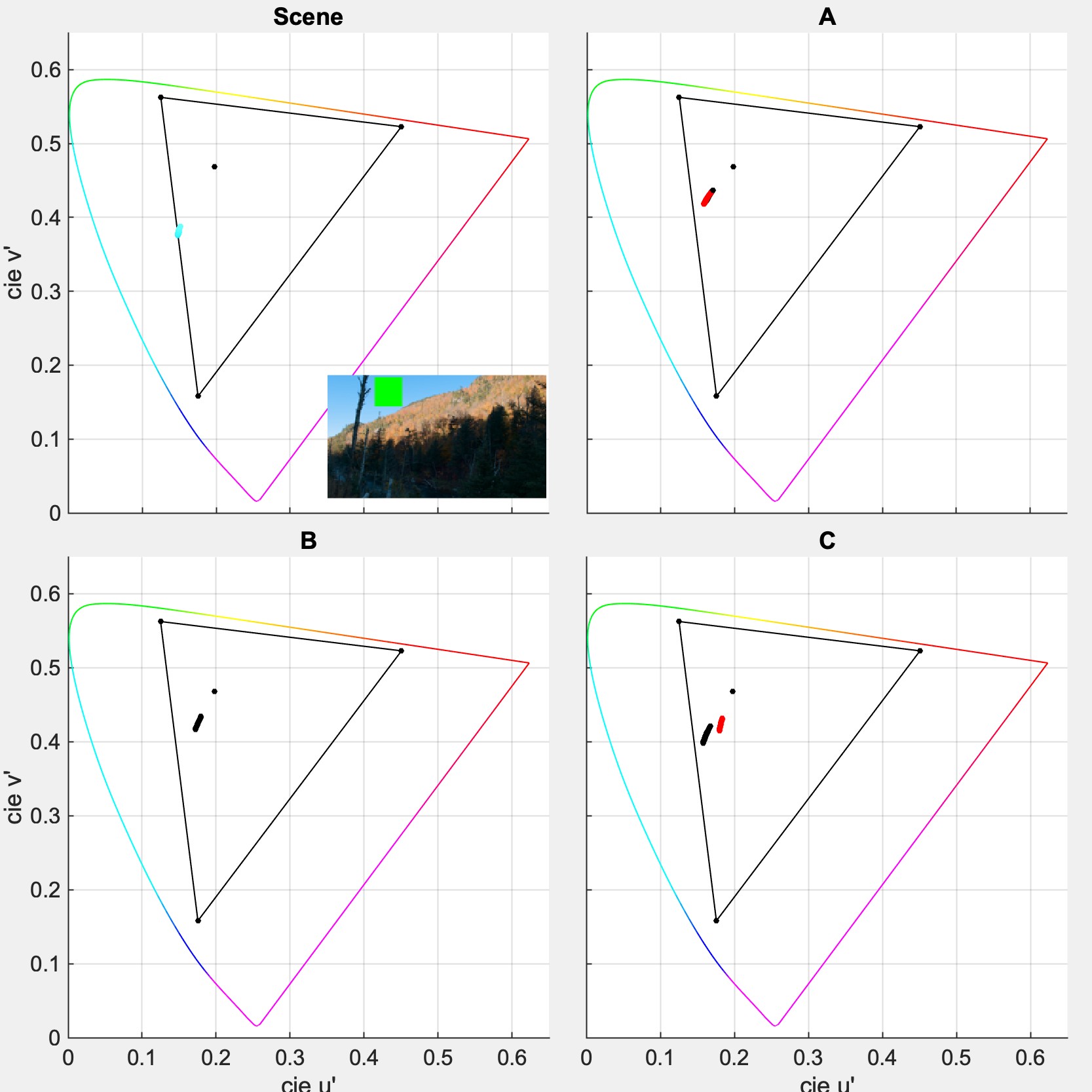
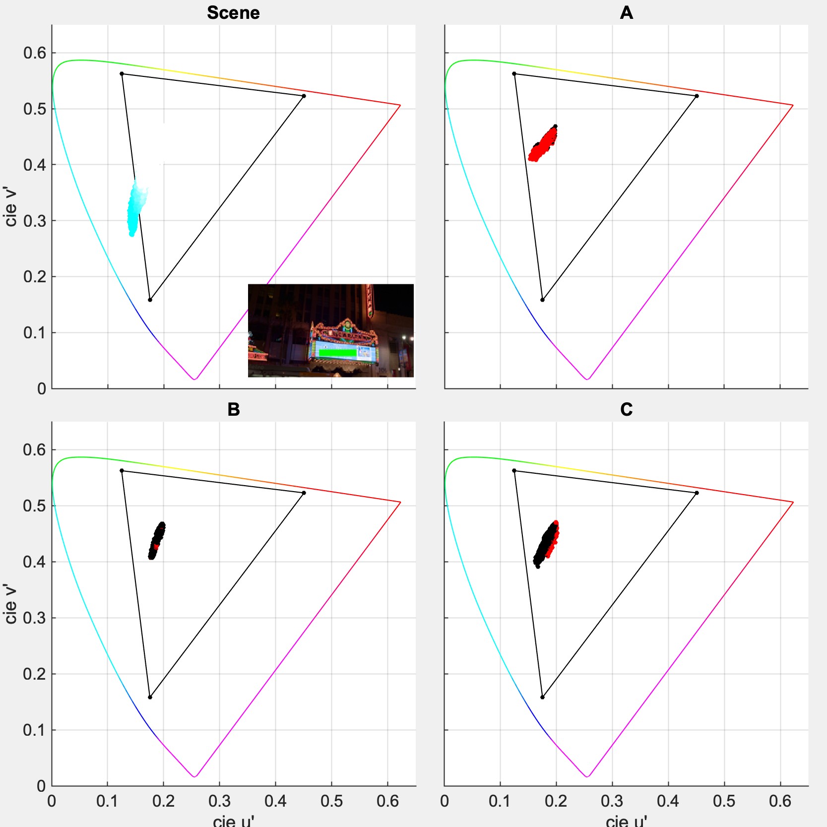
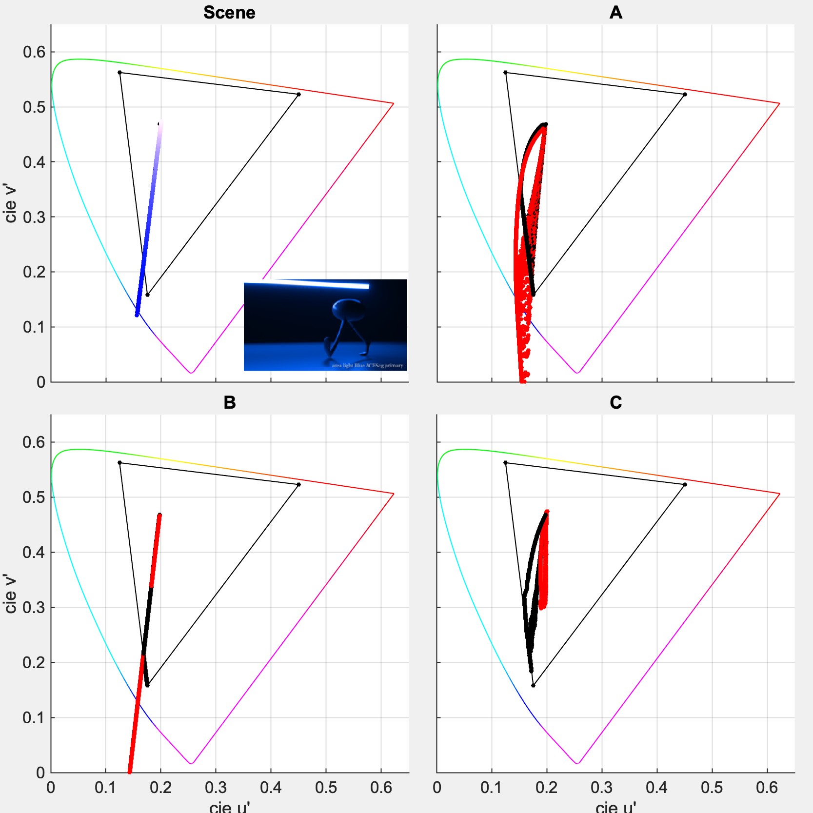
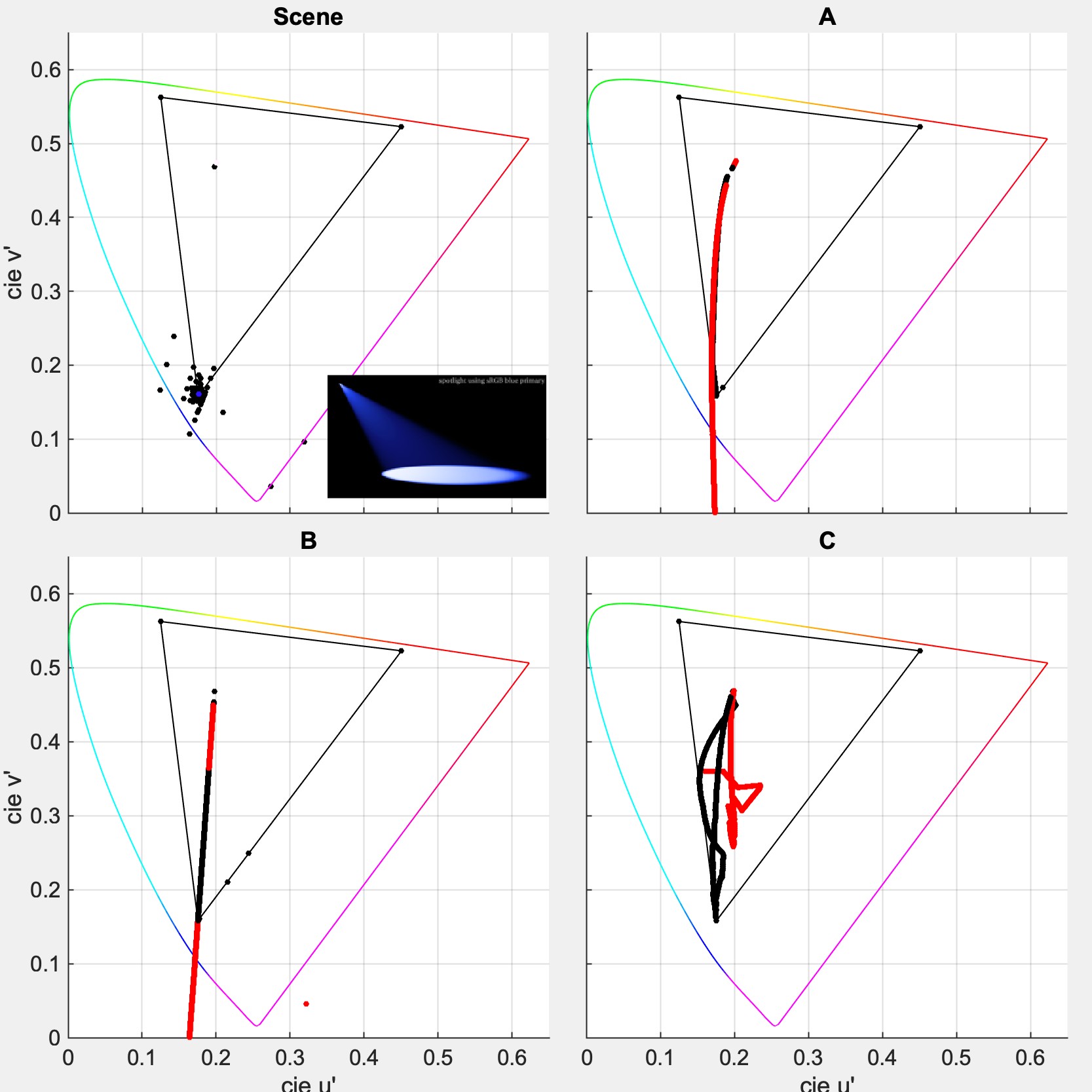
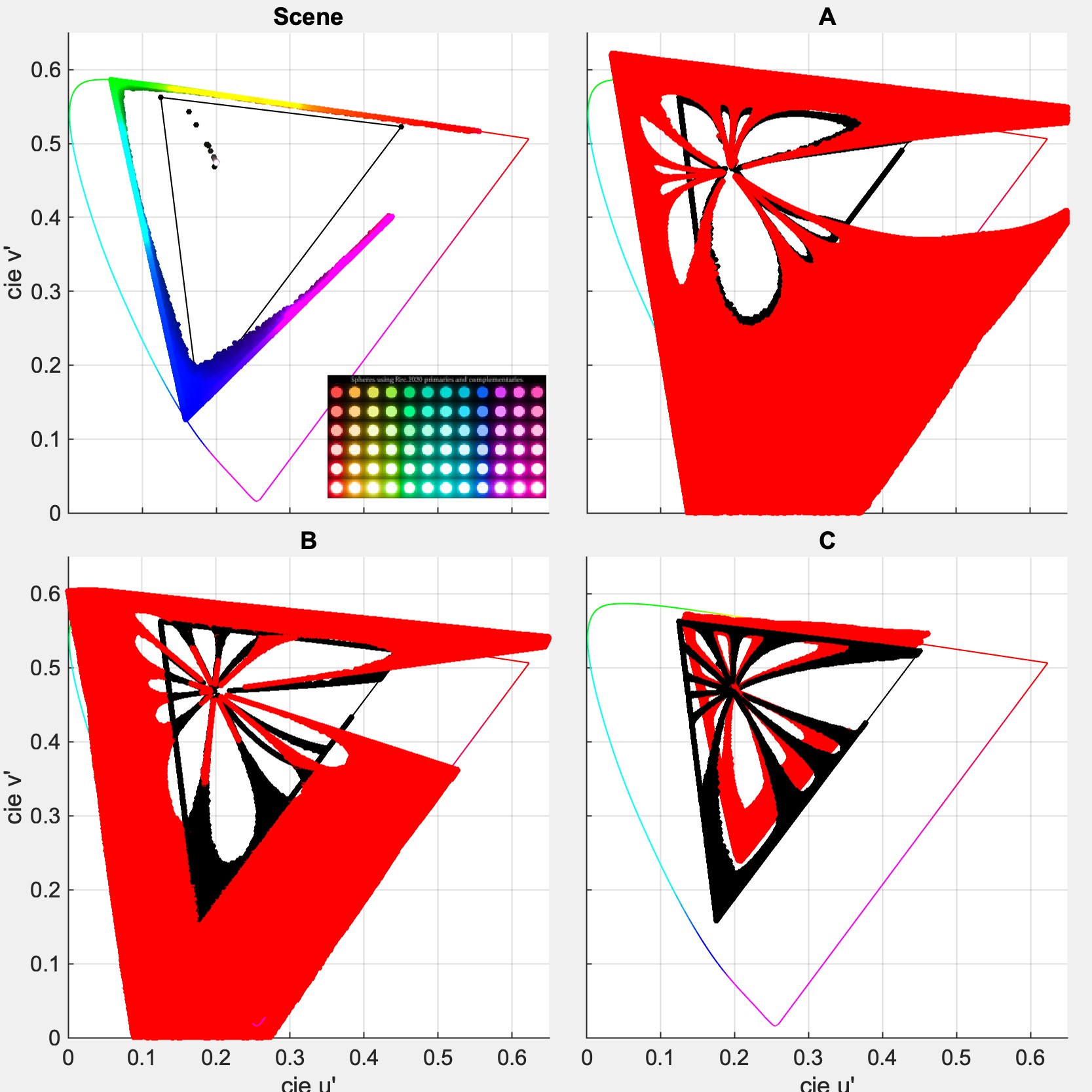
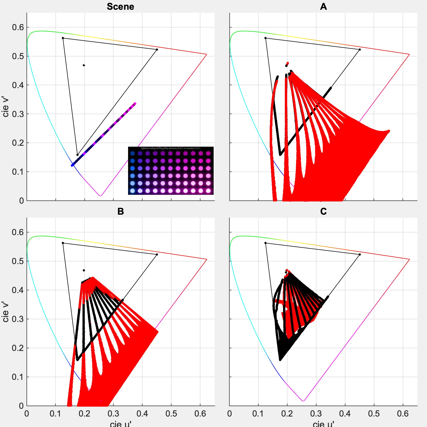
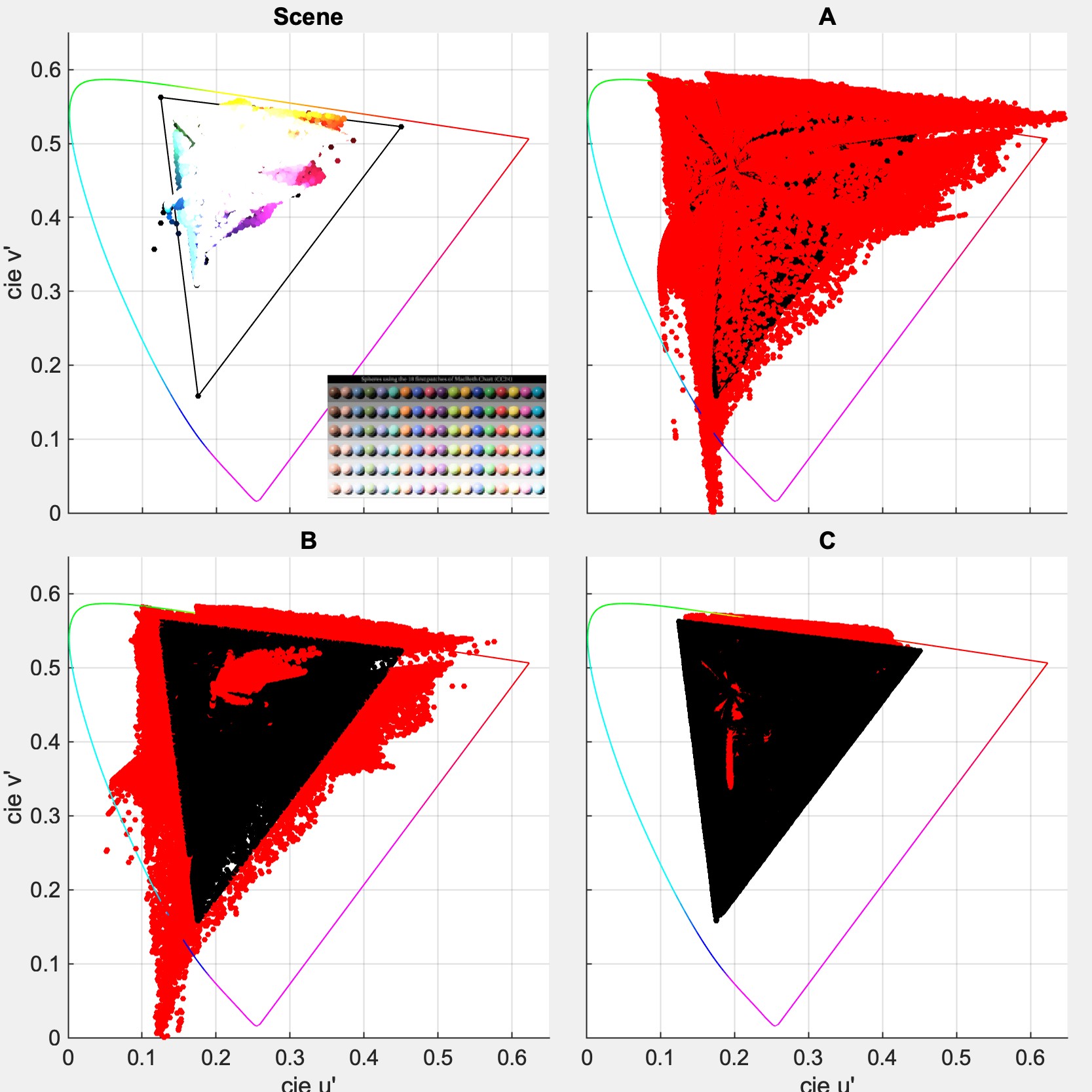
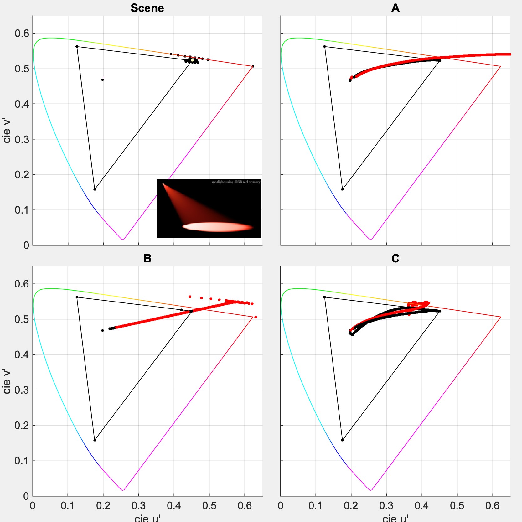
Sorry this took so long, but as promised, here are some comparisons of some of the blues and reds using the three transforms.
These plots show three things:
Note: Candidate A and B are being processed through CTL code. Candidate C, for practical reasons, is being processed using LUTs.
Candidate B is shown without the “smart-clip”. I will do a comparison of w/ & w/o smart-clip in a followup post.
I will also add plots for ramps of pure primary/secondaries of AP0, AP1, P3, and sRGB.
Some of these might need further refinement to better show what is going on.
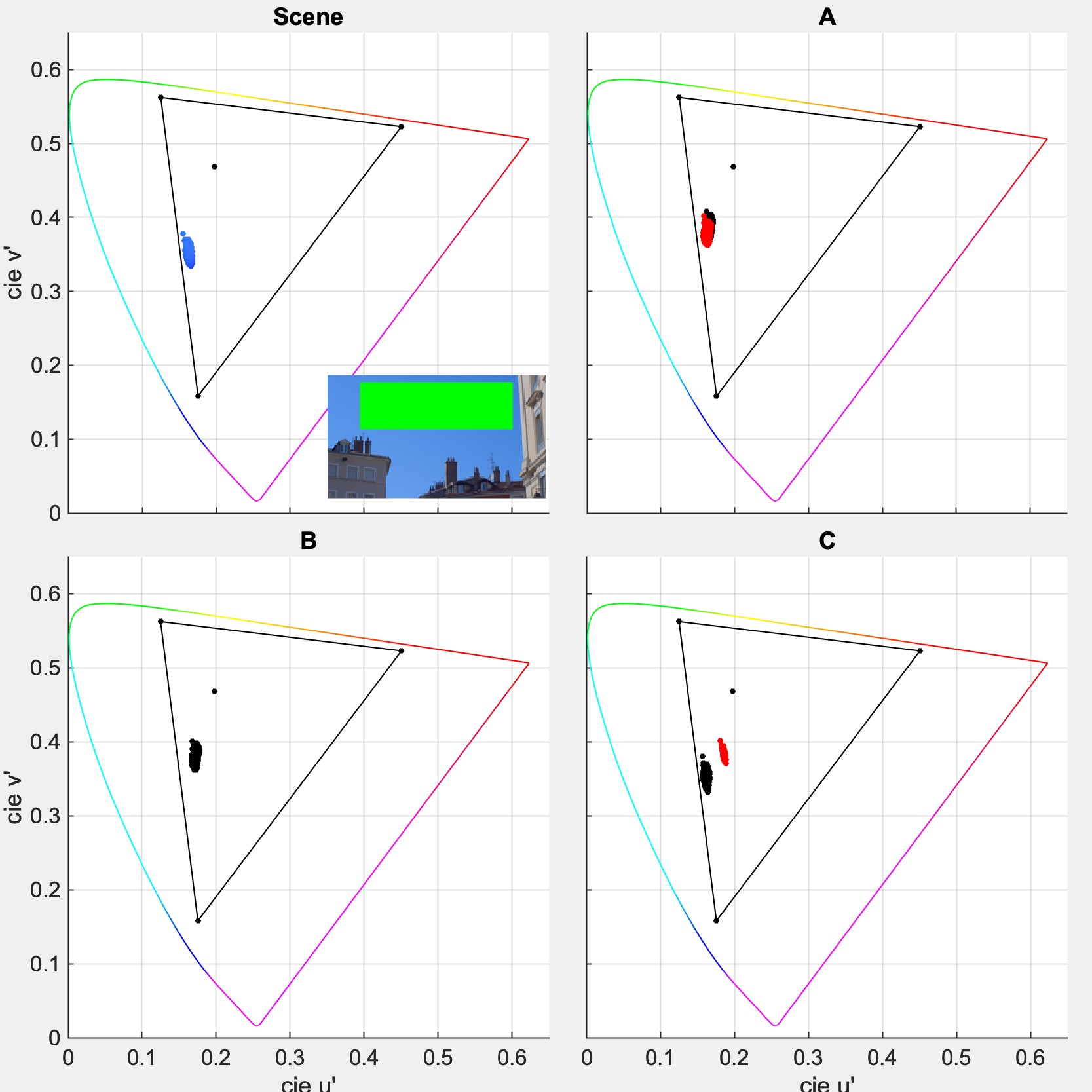
As an experiment, I also generated spokes of 31 hues evenly spaced in Oklab h, with varying L and C to make a cylinder of evenly spaced values. I then converted those to XYZ and then to ACES. I eliminated any values that fell outside of Rec709 primaries and I ran those values through A, B, and C and looked at the chromaticities before and after the rendering.
And in Oklab:
In terms of input and visualization space, what other ways might it be useful to compare the renderings?
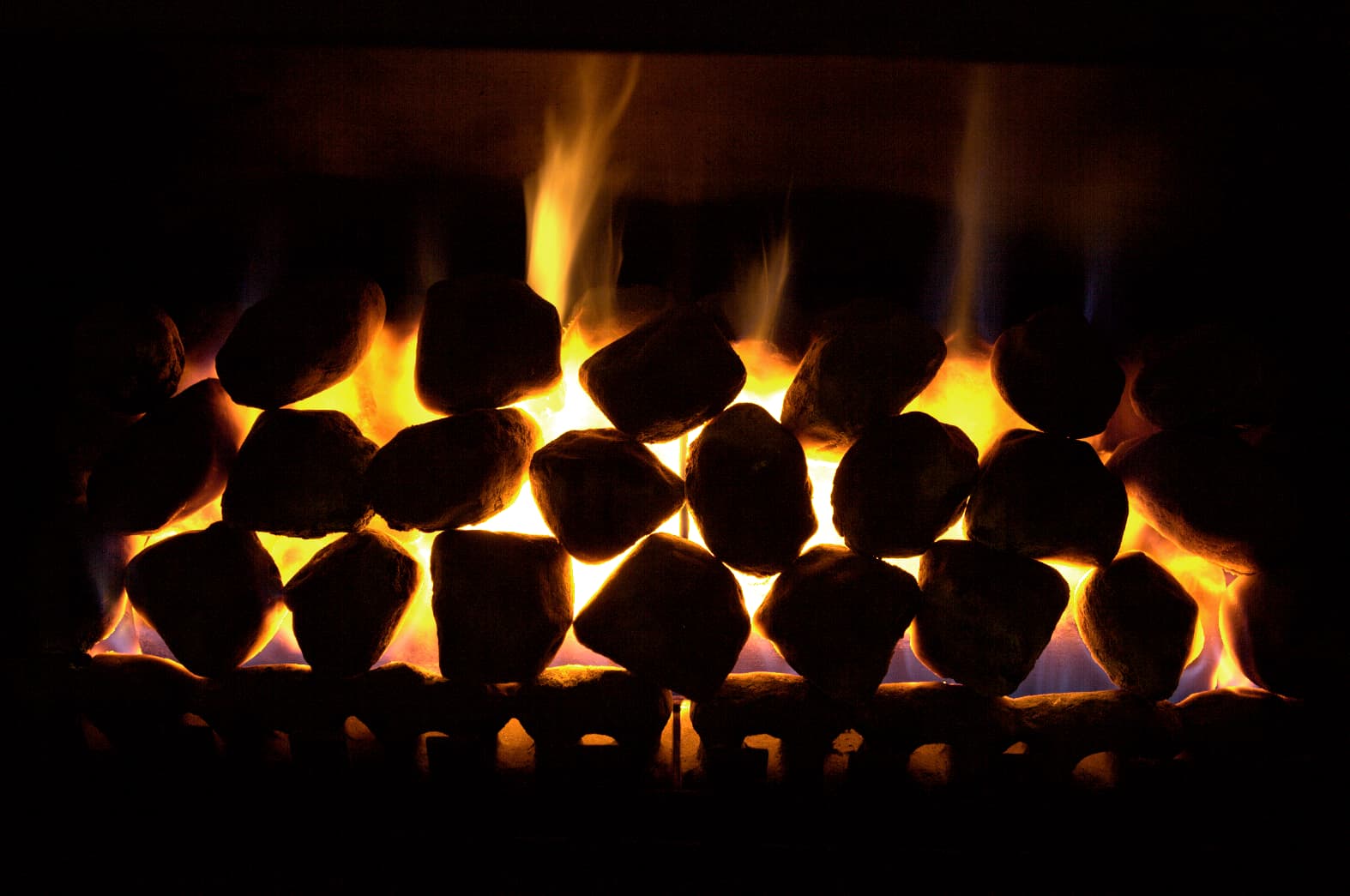
@alexfry I wanted to suggest that @Thomas_Mansencal 's fireplace EXR be added to the image set for your SDR/HDR comparisons. It makes a really useful ground truth for how real fire looks in both SDR and HDR, in contrast to a CG simulation of fire, and it shows the full range of colors temperatures - from blue to red to orange to yellow.
I wanted to also throw out there that while there has been much discussion around the possible need for a default LMT to introduce hue skews in cases like this, I’m not sure that this is needed with the current DRTs. For example, Z-CAM in HDR looks sort of monotone with the fireplace image, but simply raising the exposure (about 3 stops) on the image brings out all the lovely colors in the image right out of the box.
Note that the above image is a screen grab of an HDR (+3 stops) in zCAM, so obviously a bit gets lost in translation here, hence my suggestion it be added to the SDR/HDR webpage, perhaps with the exposure adjustment.
Added the fireplace image (0 and +3) to the bottom of the pages.
https://alexfry.github.io/ACES_ODT_Candidates_Examples/
The “Matrix + EOTF vs XXX” pages are useful here to see how it looks vs the input data (assuming you have a HDR display).