ZCAM for Nuke

Any chance you could describe what you mean by this in a little more depth?

Sure!

You got 1. exactly right.

After that you convert to the target RGB gamut. Since we compressed to a larger space, you can have colors outside the gamut though, with RGB values less than zero and larger than one. So, need some way to map those values into the [0,1] range. Just clipping to that range does OK, but will introduce some non-smoothness into your mapping. So instead you can use a curve like this to get a smooth transition near 0.0 and 1.0:

]()

Then there are some more details to not have the effect near white and black (since this would distort grayscale values) and to use the curve for both 0.0 and 1.0. The full implementation is here:

This is the difference between soft and hard clipping, when looking at the hull of the gamut approximation:

Would be nice trying this with a tighter gamut approximation also, so it touches/almost touches most of the RGB gamut corners. That would make the flat areas smaller. Haven’t had time to do that yet though.

4 Likes

For those who are interested, I have now pushed version 9 of the DRT ZCAM prototype to my GitHub repo:

https://github.com/Tristimulus/aces_vwg_output_transform

Based on the insights provided by @bottosson, this version adds a feature to apply smoothing to the edges of the target RGB cube used for finding the gamut boundary when compressing the colorfulness (M) correlate:

The result is a reduction in the color fringing that was previously observed by @jmgilbert on the Rec.2020 luminous spheres test image:

image

Since the smoothing comes at the expense of saturation at the edges and corners of the target gamut the “limit” parameter of the compression function has been reduced to compensate.

In addition the option to toggle between projecting the lightness (J) correlate towards either the lightness of the gamut cusp or SSTS mid-grey has been replaced by a slider to blend between the two instead.

6 Likes

Great work @matthias.scharfenber!

Worth also noting that the hue skew toward cyan is still present:

Notice the clumping of cyan.

1 Like

As mentioned in the last WVG meeting I have now pushed version 10 of the ZCAM IzMh DRT to GitHub:

This version is now a pure Blink script node (the Blink code is available as a separate file as well) and runs significantly faster than the previous ones.
The v10 also replaces the 2-Stage gamut compression approach with a single stage that compresses both J & M correlates at the same time towards a focal point.

I’ve also added some tool tips to the Nuke node and hopefully helpful comments to the code.

7 Likes

Jed has been working on a number of look tools, one of the more recent one’s being ShadowContrast. OpenDRT is not intended to “look good” without an added LMT, so I thought it could be interesting to show Zcam and OpenDRT + LMT side by side. The “look” consists simply of a ShadowContrast node with settings intended to approximate a similar tone scale to ACES.

Of course there are the familiar differences in the two, but I found it striking how similar they look side by side with the similar tone scales.

5 Likes

Interesting that the gradient blending is really different here:

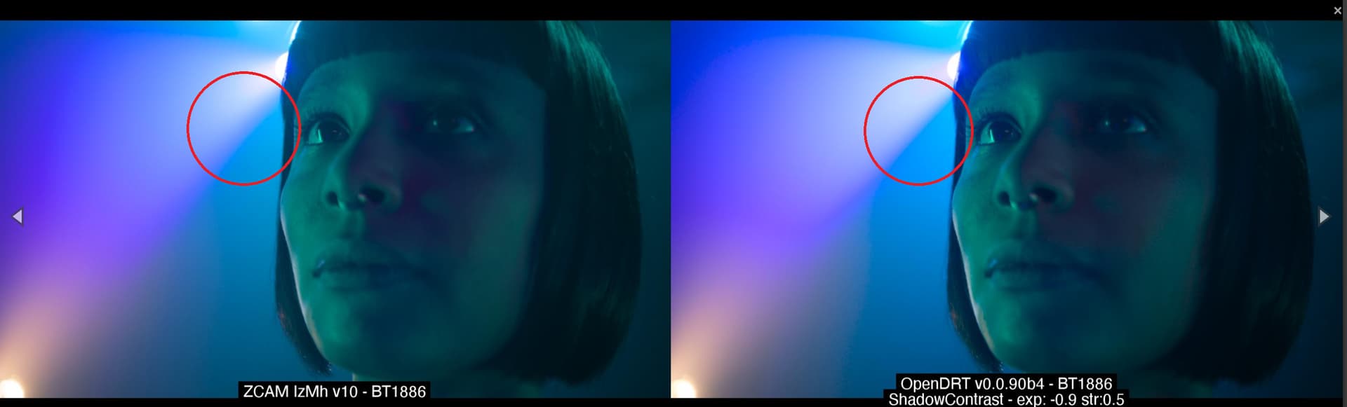
Maybe the compression does not help and produces some artefacts too.

1 Like

Thanks for those tests, there are quite interesting. I still think the biggest issue I have with ZCAM DRT is this :

We can also notice this “cyan” effect on the Light Sabers and Blue Bar. Otherwise, indeed, results are not too far apart.

Chris

I still don’t understand what “lit with ACEScg blue primary” really means . That aside …

If we say that the scene objects have the chromaticity of the ACEScg blue primary, why would one expect that to end up as being blue (e.g. rgb=[0,0,1]) in display code value space?

The chromaticity of the ACEScg “blue” primary has a hue that’s defined by JzAzBz in ZCam. We can’t see the ACEScg blue, so we don’t know the hue. Assuming we believe ZCAM works (big assumption), if one follows that hue line into a gamut that’s smaller than ACEScg and able to be reproduced on a display, that’s probably the real hue of the ACEScg primary.

1 Like

In addition to the CG renders of blue light, here’s a photo of blue light (coming from the gamut mapping test images)
zCam-JedCam_blue.05

Something else perhaps worth noting: The green dude looks less saturated in zCAM. That might be from the highlight desaturation though, rather than a hue shift.

Anyone want to explain to me how a fit model (replace the F with SH) based around a display EOTF JND experiment could ever possibly even remotely work even faintly like anything related to the HVS?

Thanks.

2 Likes

It is a hue shift in the greens toward cyan. For example:


1 Like

I’ve always thought of it that same way. Saying that a reproduction of something lit with an AP1 primary “looks wrong” is making a big assumption about what we think the AP1 primary actually “looks like”.

1 Like

I’m sorry… this is pure madness.

Imagine laying out a 2D map of the 3D earth globe, pointing beyond to the table, and speculating what it looks like.

“Hey honey… want to go to Wyoming?”

“No… let’s go north of the North Pole!”

Way out into astronaut architechturism.

2 Likes

I would use a laser-like primary such a that of BT.2020 and then we can continue the discussion whilst having everyone comfortable with the idea that this time it can be seen by the CIE 1931 2 Degree Standard Observer.

Because the Standard Observer does not see it, it does not mean that you won’t. We are using a much needed frontier, average of a few observers, because it is simpler mathematically (who wants to carry probabilities around?) when in reality it is statistically much fuzzier.

Should we instead use the probability that this particular stimulus is visible for a “probabilistic observer”, it could very well be high. I will compute that for the Asano Observers when I have spare cycles.

@ChrisBrejon: What about converting your image from BT2020 to AP0. You haven’t rendered spectrally anyway so it does not really matter. The result won’t be much different though as you might rightly so expect.

Cheers,

Thomas

Until I get to do it, here is something relevant: About issues and terminology - #7 by Thomas_Mansencal

Sorry, you are conflating issues in the same way your Asano diagram seductively creates the idea that all projections are on the CIE xy projection, as opposed to appreciating that the horizons for each observer there are singular and closed domain.

The space is bounded. Suggesting that anything exists beyond the spectral locus for the observer is absolute nonsense and rubbish.

All we have is the standard observer model, and the moment we step outside that, all bets are off and we are into nonsense land. Can a standard observer, as per Asano et al be calibrated for that specific observer? Absolutely. Suggesting that somehow the spectral locus is different and meaningful beyond the locus, as opposed to a psychophysical representation in each observer, is pure nonsense.

It’s a physical wall of visible electromagnetic radiation.

Trying to suggest that AP1 blue might be visible to some other observer is hilarious.

2 Likes

I was mistaken to use AP1 as the example in my previous post. It was a bad example.

The point I was trying to make is that there’s no reason to assume a primary in a larger RGB space should map to the primary of a smaller RGB space when converting between them. Further the hue of the larger space’s primary may very well be reproduced with a mixture of Red, Green and Blue in the smaller space.

2 Likes

This is a discussion I tried to bring up way back at the “gamut” mapping VWG way back when. What is a reasonable and sane approach here for getting values to a working model?

  1. Perceptual “hue”.
  2. Tristimulus linear-energy-like.

Could the working space mapping be different and subject to different requirements to the image formation mapping?

2 Likes

Yeah well, no. The CIE xyY projective transformation is valid for any observer. You can also design a transformation that maps an observer to another.

The space is indeed bounded but there are as many spaces as there are observers, for the same reason that there is a sensitivity space for every single camera.

Again it is a wall for the particular observer you use, nothing says that a stimulus this observer cannot perceive will not be seen by another one. We have plenty of observers, e.g. the Individual Observer, even the standardised ones, e.g. 2012, proving it is the case.

If you make the border probabilistic instead of an average/mean, you can come up with a probability that it can be seen by a distribution of observers. Put another way, we are only considering the central slice of the distribution of observers that served to build the Standard Observer.

You then could certainly find a value that is visible for some observer and that is mapped exactly where AP1 blue is located for the Standard Observer. We do that all the time with cameras and, surprise, many values are mapped outside the spectral locus!

Cheers,

Thomas

1 Like