ZCAM for Nuke

alexfry · November 3, 2021, 5:44am

After Alex Forsythe’s suggestion about using ZCAM in last weeks meeting, I thought I better try and get my head around it. Generally I find the best way to do that is to try and make it work in Nuke, so I’ve given that a crack.

I’m not going to pretend I fully understand what’s going on here, but hopefully there is enough here for people to have a play around with, or improve on, or integrate into something larger.

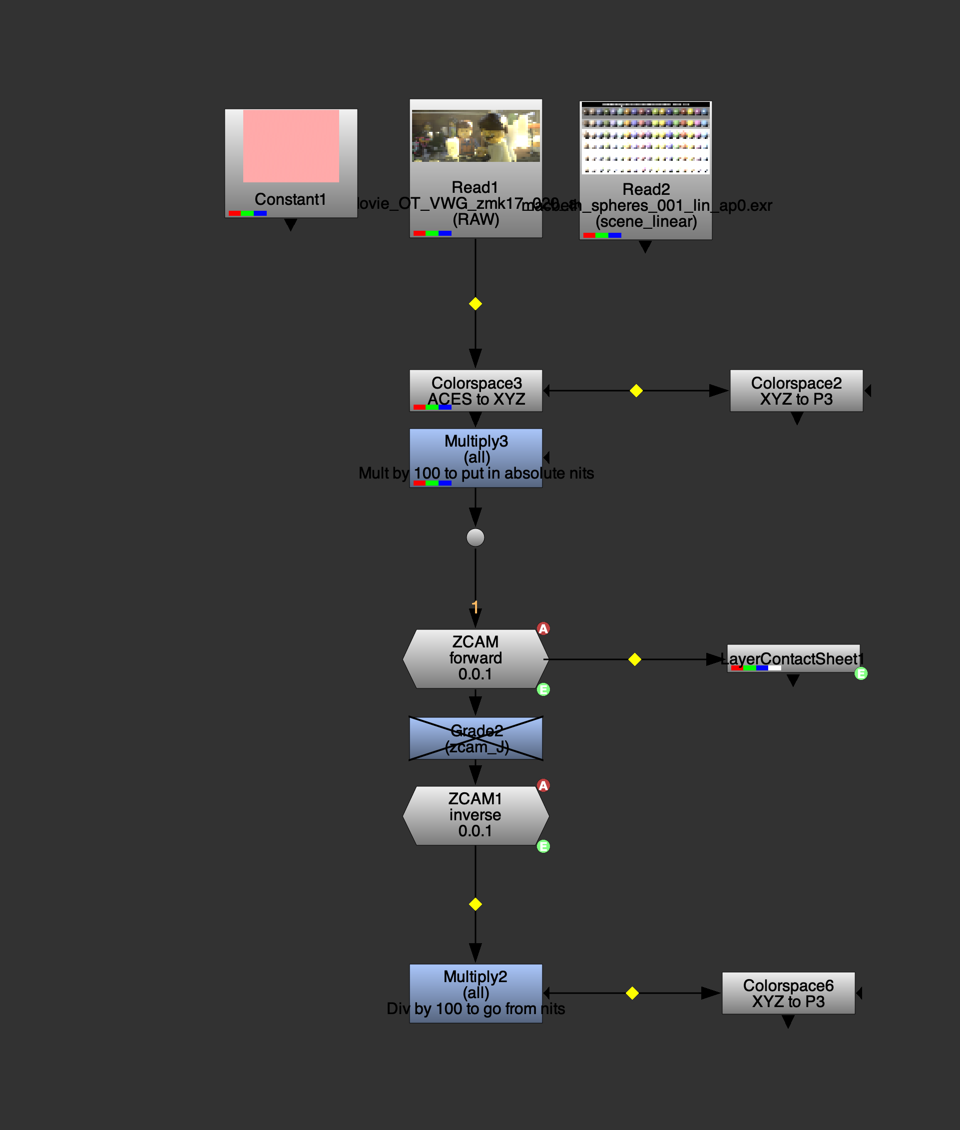
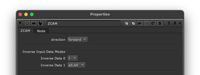
The node has two modes, forward and inverse

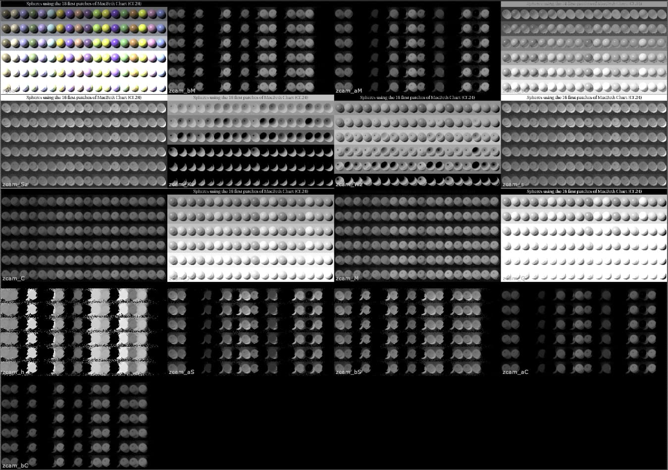
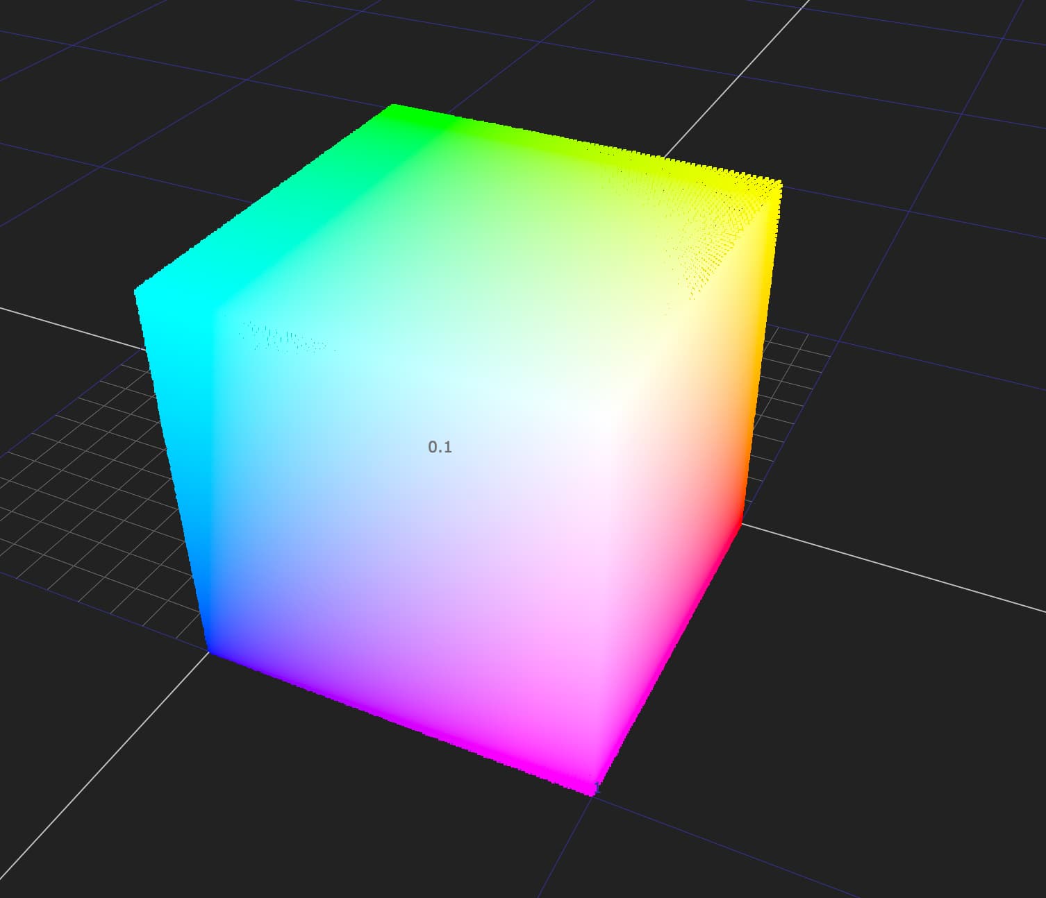
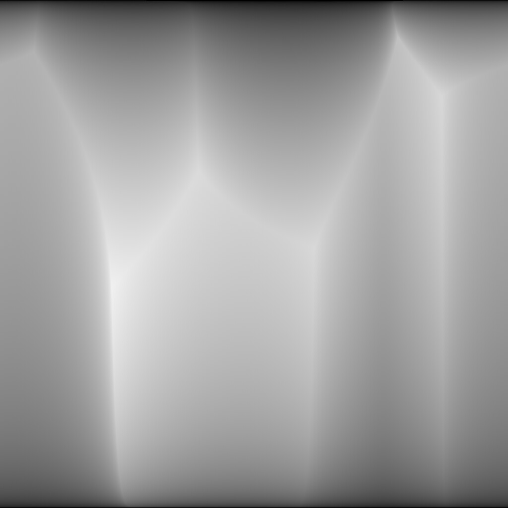
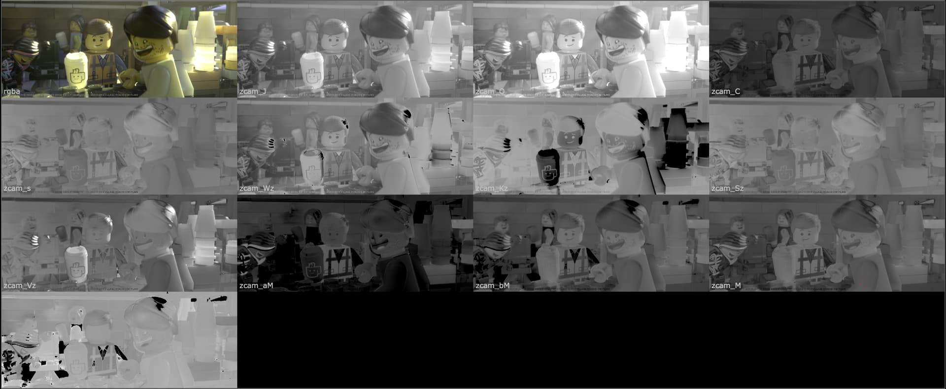
forward will dump as many of the attributes as I could produce into layers with a zcam_X. naming convention (same info in each layer’s rgba channels), whilst leaving the xyz data in the main layer. You can view them by looking at the stream with a LayerContactSheet node.

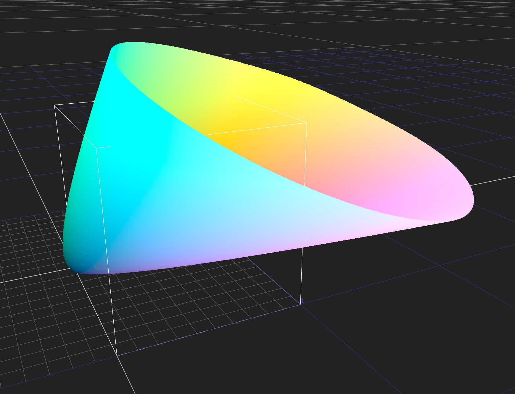
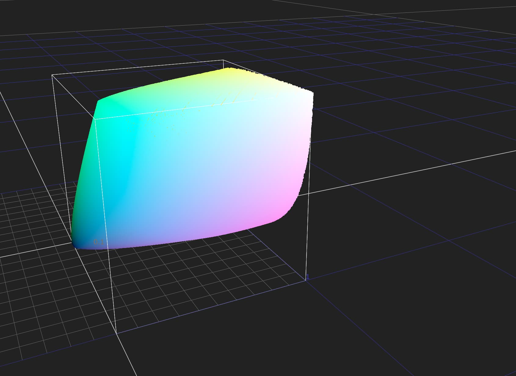
inverse will reconstruct xyz, but only using the J,aM,bM attributes (This could/should change in the future).

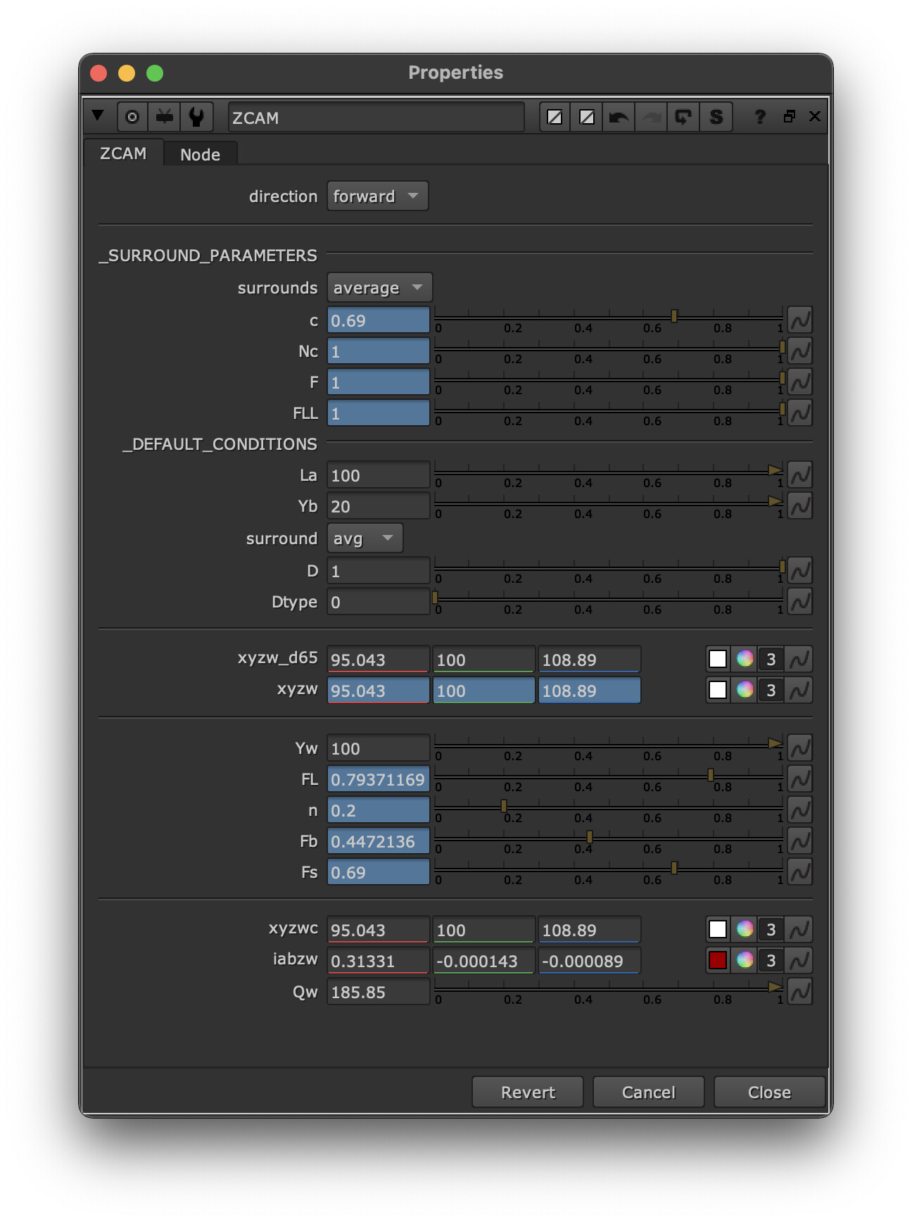
There are a bunch of params to play around with, the only ones I’ve really touched so far are the different surround constants (which seem to do… something).

The guts of the node are pretty gory, but it seems to do what I expect, forward → inverse will behave as a null op, and pushing around the zcam_J layer in the middle will push things around. Hopefully there is some value here for people who want to experiment, and try and understand it (which is all I’m attempting to do here)

I’ve based my implementation on the python version found in luxpy here:

github.com

ksmet1977/luxpy/blob/master/luxpy/color/cam/zcam.py

# -*- coding: utf-8 -*-
"""
ZCAM: Jzazbz-based color appearance model
=========================================

 :_UNIQUE_HUE_DATA: dictionary with unique hue data 
            
 :_SURROUND_PARAMETERS: dictionary with surround param. c, Nc, F and FLL for 'avg','dim' and 'dark' conditions

 :_NAKA_RUSHTON_PARAMETERS: | dictionary with parameters (n, sig, scaling and noise) 
                            | for the Naka-Rushton function: 
                            |   NK(x) = sign(x) * scaling * ((abs(x)**n) / ((abs(x)**n) + (sig**n))) + noise

 :_DEFAULT_WHITE_POINT: Default internal reference white point (xyz)

 :_DEFAULT_CONDITIONS: Default CAM model parameters 

 :_AXES: dict with list[str,str,str] containing axis labels of defined cspaces.

 :run(): Run the Jzazbz-based  color appearance model in forward or backward modes.

This file has been truncated. show original

Thomas_Mansencal · November 3, 2021, 8:38am

Nice! I haven’t poked at it too much but it seems like you don’t have the first chromatic adaptation step, i.e. Step 0.

Because it is under-documented and I spent a bit of time trying to get the numbers matching the Supplemental document, you need to effectively do a Von Kries chromatic adaptation but it needs to include the degree of adaptation D that can be computed from the CIECAM02 equation. Because the values fed to the model are absolute, you will also want to normalise the D65 whitepoint WRT the reference whitepoint XYZ_w. There is no documentation again on how to do that, but XYZ_{D65} / Y_{D65} * Y_w seems to do the job when doing the chromatic adaptation.

The Colour implementation is not finished but getting there

Cheers,

Thomas

alexfry · November 3, 2021, 10:07am

Ahh yes! I forgot to mention that.
I’m assuming you’ve already got your data in D65.

alexfry · November 4, 2021, 3:17am

I’ve made some updates to allow the forward mode to output aS and aC (as well as aM), and added support for multiple reconstruction modes to the inverse path.

The first version only supported J, aM, bM.
It now supports J or Q ( Brightness or Lightness)
Along with aM/bM, aC/bC, aS/bS and M/h or C/h

This is based on what I see in the luxpy implementation:

        :outin:
            | 'J,aM,bM', optional
            | String with requested output (e.g. "J,aM,bM,M,h") [Forward mode]
            | - attributes: 'J': lightness,'Q': brightness,
            |               'M': colorfulness,'C': chroma, 's': saturation,
            |               'h': hue angle, 'H': hue quadrature/composition,
            |               'Wz': whiteness, 'Kz':blackness, 'Sz': saturation, 'V': vividness
            | String with inputs in data [inverse mode]. 
            | Input must have data.shape[-1]==3 and last dim of data must have 
            | the following structure for inverse mode: 
            |  * data[...,0] = J or Q,
            |  * data[...,1:] = (aM,bM) or (aC,bC) or (aS,bS) or (M,h) or (C, h), ...

The controls only effect the inverse mode, as the forward mode still just dumps everything out.

As @Thomas_Mansencal noted, this still does not contain the CAT to D65 step.

Thomas_Mansencal · November 7, 2021, 6:34am

This is actually more complicated than I thought, as we have the model implemented in a PR, here are some relevant notes:

Safdar, Hardeberg and Luo (2021) does not specify how the chromatic adaptation to CIE Standard Illuminant D65 in Step 0 should be performed. A one-step Von Kries chromatic adaptation transform is not or transitive when a degree of adptation is involved. Safdar, Hardeberg and Luo (2018) uses Zhai and Luo (2018) two-steps chromatic adaptation transform, thus it seems sensible to adopt this transform for the ZCAM colour appearance model until more information is available. It is worth noting that a one-step Von Kries chromatic adaptation transform with support for degree of adaptation produces values closer to the supplemental document compared to the Zhai and Luo (2018) two-steps chromatic adaptation transform but then the ZCAM colour appearance model does not round-trip properly.
Step 4 of the inverse model uses a rounded exponent of 1.3514 preventing the model to round-trip properly. Given that this implementation takes some liberties with respect to the chromatic transform to use, it was deemed appropriate to use an exponent value, i.e. 50 / 37, that enables the ZCAM colour appearance model to round-trip.
The values in the third column of the supplemental document are likely incorrect:
- Hue quadrature H_z is significantly different for this test, i.e. 47.748252 vs 43.8258.
- F_L as reported in the supplemental document has the same value as for L_a = 264 instead of 150.

nick · November 10, 2021, 4:48pm

Am I missing something? Does it not simply specify CAT02?
zcam_step_0

Thomas_Mansencal · November 10, 2021, 5:58pm

Well, a simple Von Kries transform with CAT02 does not work because the illuminant values are absolute, i.e. it will scale the input tristimulus values in a non desirable way. At which point you are opening a can of worm: Is it a Von Kries transform or the CIECAM02 transform from which CAT02 is originated? Should it support degree of adaptation which cannot be inverted with a one-step Von Kries transform? And so on…

Alexander_Forsythe · November 10, 2021, 7:16pm

I’m dealing with similar complexities on my end.

Other issues that I’m not completely sure how to deal with are the default parameters for our application.

Regarding round tripping, would it make sense to slightly alter the model from the paper’s description so it round trips, then retest against the LUCHI dataset to see if it significantly impacts the color appearance predictions?

alexfry · November 11, 2021, 12:45am

Repo has now been updated with the bodged together ZCAMishDRT I showed in the meeting today.

jmgilbert · November 11, 2021, 4:22pm

For the code-minded ones, here are some ZCAM Shadertoys : https://www.shadertoy.com/results?query=zcam

They set sRGB reference white to 200 nits in their calculation which really makes sense.

Thomas_Mansencal · November 12, 2021, 9:00pm

As it currently stands, the Colour implementation roundtrips perfectly with the two-step Von Kries transform from Zhai et al. (2018) and the slight exponent change. I don’t think it would change any predictions as the values are really close to the supplemental paper. I’m still meant to contact the authors, been a hectic week down there!

alexfry · November 23, 2021, 3:32am

Just playing with a few ramps and gradients here.

The Image below represents:

J ramping from 0 → 100 in the y axis.
M at a constant value of 25
h ramping from -180 → 180 in the x axis

Which then passes from ZCAM (scaled down by 100) → XYZ → sRGB (display linear)

When plotted in 3D it looks like this (the cube is 0.0 → 1.0):

As (sort of) expected, the flat plane at the top of the cone seems to intersect the 1.0,1.0,1.0 corner of the cube.

Although it does not form a circle centered on that point.

The interesting lump around yellow can be seen here.

My assumption is the swelling at the bottom is the model attempting to maintain (M) Colourfulness as (J) Lightness drops. Pushing values that aren’t particularly saturated in absolute terms outside of the sRGB display gamut volume.

ChrisBrejon · December 2, 2021, 6:10pm

Hey @alexfry

sorry to bother you but I have tried to download ZCAMish DRT from your github and the nuke scripts I have found were a bit complex.

I am not sure where to read my files and where to set my viewer honestly. If you have ever time to have a quick look, thanks !

Chris

alexfry · December 3, 2021, 4:24am

Sorry Christophe, that version is a bit of a spider web brain dump.
It’s not well setup at all, it just works (barely).

Hopefully I get a version out there that’s a bit more sane soonish.

alexfry · December 3, 2021, 6:37am

OK, so the main thing I’ve been thinking about lately is how to deal with the fact ZCAM doesn’t know or care about your display gamut, and therefore is throwing values all over the place as you move things up and down.

The animated gif below shows the same ramp used above:
x = -180 → 180 in h
y = 0 → 100nits in J
And time is running from 0 → 100 in M

Anytime any channel in sRGB drops below 0, or goes above 1, I’m flipping to black.

sRGBgamutBoundGif_v001

Once I have this, I’m doing a looping Over operation (1024 steps) to build up an image that contains the maxium M value for any J and h combination (under 100nits). Which gives me an image that looks like this:

So despite being stored as J,M,h values, when visualed in 3D (flipped back into sRGB), this forms a limit cube.

So now I have an image that effectivly stores the max M value for any given J/h combination:

I can treat it as a 2D LUT, and take something like this image, which is 0->100nits, with an M of 33

And do a soft clip of the M channel, based on the max M availible in the sRGB volume.

Now this soft clip is currently pretty crude, but it does do the main two things I want, which is deal with the negs down on the bottom left, and the big excursions above 1.0 when I ask for M values of 33 at 100nits (which clearly isn’t possible).

The approch I’ve taken here is clearly not suitable for real-time work. But I’m just trying to make it work for now

So now the flow looks like this:

ACES → XYZ → ZCAM → Apply SSTS style 1D curve to J → softclip M to sRGB gamut boundry → convert to XYZ → sRGB → inverse EOTF

Below are a series of images showing how it all adds up.
ZCAMishDRT - OpenDRT - ACES 1.2
3 Stops down
Normal exposure
5 Stops up

Results are a mixed bag, some wins, some losses. But interesting none the less.

ACESCentral seems to be scaling them down, so the full rez ones can be found here:

alexfry · December 3, 2021, 11:07pm

I’m currently trying to understand where the swings toward cyan are coming from in extreme blues and greens. My suspicion is that the misalignment of AP1’s primaries to Rec709 primaries, when pulling M values back towards the whitepoint, is causing the shift.

For instance, a pure AP1 green ends up with a significant amount of blue in it when it lands along the 709 boundry.

I’m not certain, but I think this is what’s causing the effect below:

Same -3 0 +5 comparison as above:

nick · December 5, 2021, 12:59pm

Fascinating stuff. I’m trying to visualise what the AP1 green primary looks like. It must be pretty close to the colour of a 532nm green laser. Has anybody got one of those to hand, and able to compare it visually with Rec.709 green? Maybe it is a bit bluer…

ChrisBrejon · December 5, 2021, 3:23pm

Maybe ! But then how could we explain the fact that blues also look “funky” ? Because it is not only happening in the greens but also blues… And the ACEScg blue primary and the BT.709 blue primary are not that far apart ? I have absolutely no idea why would such a thing happen though…

A couple of more things :

Excellent work ! It is really really awesome that you are trying to tackle a DRT based on ZCAM and that you were able to provide so many examples both on CG and “live-action”.
A few frames show a weird “over-saturation” in their highest exposure (for instance, on the left-screen black character of the Lego one and on the “ceiling” of the Cornell box).
Interestingly enough, this “over-saturation” towards yellow (?) is also noticeable in the lat-long HDRIs around the sun area. Maybe something to investigate.
CG frames using a blue ACEScg primary in their main light source are the ones that look “weirder” to me. For instance, the one with the little ball character and the ones with the volumetric spot lights.
I find it super interesting to compare the sRGB blue primary and the ACEScg blue primary on the volumetric spot lights´ frames. The ACEScg one looks quite desaturated and almost green… Something funky going on !
You can observe the exact same behaviour on the spheres´ images using BT.2020 and ACEScg primaries.
One thing though that I thought was pretty on point is how “Mery” (the female character in the Light Saber´s image) looks. I thought the ratio “Brightness/Saturation” (omg, I am butchering the words… Sorry !) was pretty good-looking.
I also thought that most of the live-action examples, including the cars´ ones looked really good.

Nice work ! Thanks for taking the time to experiment things.
Chris

alexfry · December 5, 2021, 9:03pm

I think it’s the same thing.
When you look at the line running from the AP1 blue to D65, the point where it crosses the 709 gamut boundary is actually quite a distance along the line back towards green.

Alexander_Forsythe · December 5, 2021, 10:23pm

I think it’s important to not necessarily think of these colors as a set of RGB values relative to a scene referred space and an output space.

A straight line in CIE xy from an ACEScg primary to a white point isn’t going to be a line of constant hue in scene space. To determine a hue linear set of CIE xy values with varying Chroma (as defined by Zcam / JzAzBz), convert the ACEScg primary in question of JCh then vary C and convert back.

If you take that line and go from the colorimetry associated with scene to colorimetry associated with the output it’s the corresponding colorimetry required to produce the same perception that was elicited in a viewer in the scene (gamut considerations aside). It’s not going to make the scene colors map a straight line from the display primary to the display white point, nor should it. Again, I think that’s the danger of thinking of the scene space as a set of RGB values in this instance.

Rather than produce RGB ramps in ACEScg, I think it’d be more useful to ramp something like the XYZ values of a macbeth color checker in Chroma and look at that.

Here’s a colab.