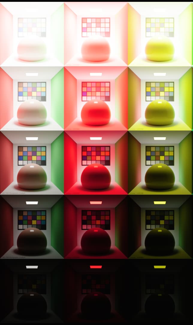
A room illuminated by Yellow Laser (or any narrow band source) probably should look uncanny.
No unfiltered LED can currently produce even a moderately narrow band in that part of the spectrum so it is unlikely that you would ever encounter such illumination.
Sodium Vapor is close, and if you have ever been in a room with only that source it is very strange indeed, an open flame can appear black!
What I would call reflective or transmissive yellows (the kind we likely evolved to discriminate) are essentially white with a little absorption in the shorter/blue part of spectrum.
One could argue that our response to Yellow is just a blueness detector, and that the yellow appearance in a rainbow or through optical diffraction is just an artifact.
To demonstrate this point, you could entirely remove the “yellow” part of the spectrum between 565/570nm-580nm from a white light source with a notch filter and still get a pretty good yellow. This does not really work with other colors.
With that said I wouldn’t press the point too much, just a curious observation, and may not be relevant to what you are observing, since the yellow Hue in the picture is a result of the camera/observer response to those wavelengths regardless of where they are positioned.
I still think it has a little to do with the illumination coming from behind the sphere, the yellow of the sphere is a little dark compared to yellow patch in the color checker.
None of this is to say that there isn’t a problem with the current DRT, I am sure there is, since it is still unfinished and open to revision, which is why we need to be careful on how we are evaluating what the exact problem is.
I am not sure how useful this claim is. The colors are what they are based on the particular intensity of a particular band with a particular observer, whatever the result is the result.
Is there an error in process?
What should it look like?
Thomas has clarified his calibration and Alex has shown an alternative normalization, so what other alternatives could be recommended?
It’s a picture. Not a simulacrum. None of the trends that occur in a picture are even remotely “as though we are standing there.”
It’s a picture.
Balance out any illumination to a global frame of achromatic. There will be maxima near 575 and 500.
There is a good bit of research on the layering cognition principle. Even reading the Kingdom paper would be prudent as an entry point.
Alex’s normalization reveals this. Yellow should not end up “darker” in terms of luminance. This is indeed an error in process.
Anyone who has attempted a luminance mapping knows this; we don’t map the luminance and then also cognize the chromatic strength at that mapped level. It’s a double up. These sorts of plots are telltales that the error is one of process.
As a default assumption, for “generic” pictures, it is very reasonable to suggest the cognized level should pattern after luminance. Global frames of achromatic follow this pattern. Try mixing the yellow with the blue and you’ll understand why.
We already know that the luminance and the chrominance combine for “total force” of a given global achromatic frame. These principles are deeply rooted in visual cognitive differentials, and are present in the display you are looking at. Why is BT.709 yellow at 92.78% luminous force countered with a mere luminous force of 7.22% BT.709 blue? Because BT.709 blue carries a differential of 12.85 times the “chromatic” force of BT.709 yellow.
Alex’s normalization is in fact close to a reasonable test case. And it’s pooched.
While this is a general rule, I don’t think it applies to narrow band sources.
Here is the CIE (2008) physiologically-relevant luminous efficiency function for photopic vision with an actually existing 594nm FWHM 10nm laser Bandpass filter and the resulting product, which peaks at about 591nm.
I don’t know how it could have a maxima at 500nm or 575nm if there is little or no energy in that range.
Again, none of this is to dispute that something might be “off” with the current DRT candidate.
I also suspect some problems in the Yellows, as Pekka has mentioned that region needed some extra attention in the past and was desaturating more than expected with certain functions.
Just don’t want to target the wrong problem, if something else can explain that problem.
Check out the image also in Rec.2100 and the same can be observed.
With this image we’re observing gamut mapper’s behavior. By changing the compression the behavior can be changed (and can be easily improved). I also think that the cusp-to-mid-blend as well as the focus distance should be hue dependent (and not just cusp J dependent) so that for example yellow with a high cusp J and cyan with a high cusp J can still be treated differently. This could be done with a hue dependent curve quite easily. (I brought this up in Feb 1st 2023 meeting and v27 had something like that going for it but it was decided it was the “wrong domain” to do it in, but I still think it’s needed.)
We have to remember that the totality of the Standard Observer projection is effectively a rather ropey presentation of an attempt at neurophysiological signals. Sadly, our visual cognition system does not appear to work the way that the orthodoxy of colourimetry would present, but let’s take it at face value.
We have a globally adapted centroid under the model. That is, when we think about the “map”, the outer locus horseshoe corresponds to projected coordinates based on the aforementioned centroid; all coordinates that represent the infinite series of “spectra” are carefully balanced such that all opponents cancel polarity on the illuminant E assumption. If we shift the illuminant, we shift the Observer itself, however the general conceptual outline holds.
We can validate this by summing the CIE XYZ “signals”, and we will see, plus or minus some historical notes not worth getting into, the sum is very close to the Illuminant E coordinate centroid.
I don’t think this is a useful construct here. The luminous efficacy function is a very broad and loose attempt at gauging the response of the Protan + Deutan response. All it can inform us is of the relative luminance sensitivity of the infinitely small slice at that band. It is not representative of the “stasis” of balance of the standard observer.
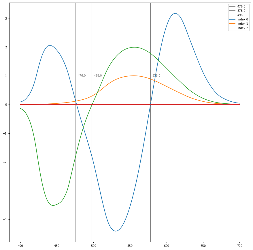
Imagine drawing a line through the achromatic centroid that bisects the CIE xy locus on opposite sides of the centroid. If we calculate the chrominance of the bisection points of the Sample and the Complement, we can calculate the ratio of “energy” required to “balance” it at the centroid. I’ll skip the math, but if we do this for an N series of bisections, we arrive at a plot similar to the following:
Note the characteristic “minima” near 575nm? This happens to be the point of maximal chrominance to maximal luminance in terms of the underlying neurophysiological signals. We can unfurl this further in terms of the correspondence of the three basis differentials as outlined by Judd1.
To understand why there is a classic peak at 575 nm, it requires understanding that the position marks the point of maximal chrominance of the opponent signal, which equates to minimal chrominance and maximal luminance of the Protan + Deutan +/- Tritan component, identified as “Index 0” in the above Judd plot. This peak is a dip in chrominance, which has been coined “Sloan’s Notch”2.
TL;DR: We have to think about the CIE xy model as a whole, not individual parts. And that “whole” is based on the underlying assumption of a “flat” energy, or Illuminant E, upon which the totality of the range of visual sensitivity is balanced against that centroid. Or at least that’s the assumption baked into CIE xy.
It’s a fair question, although I believe it’s both. And due to a double up logic.
The underlying assumption that one should “map” the “lightness” of a given sample is why there is a double up.
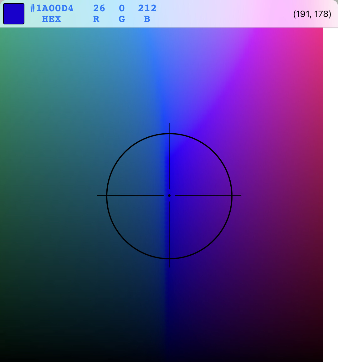
If we reverse engineer BT.709 for pedagogical purposes, we can think about the opponents of the pure BT.709 “red” and the complementary “green” and “blue” combination of “cyan”. If we use luminance here instead of the rather goofy “J” component of these sorts of models, we end up with 21.26% as a weight. If we map that down on some curve, we are now disrupting the actual position it is required to function properly in the stasis of BT.709. This leads to these sorts of goofy plots, such as this one from the equally silly OKLab:
This is a broken plot. It’s hard to spot, but it makes perfectly good sense once the demon in the detail is spotted. Here the “up down” mechanic is loosely luminance, or some non uniform variation. Doesn’t matter. The point is, the maximally pure blue is mapped way down. This is the wrong position. Why? Because these sorts of plots are luminance biased. As in an isoluminant projection that is utterly ignorant of chrominance. When chrominance and luminance are combined in proper magnitudes, we end up with the inevitable “balanced” system.
It took me a long time to realize the double up, and I’ve seen many wise minds succumb to the error! Yet it’s right there. The error is effectively a double LUT, where the first pass is the error mapping of luminance, ignorant of chrominance force, and the second pass is the one that happens cognitively.
When we properly balance luminance against chrominance, we end up with… wait for it… something that is… in every display medium and camera plane system ever engineered. It’s a basic RGB model. Or CIE XYZ. Or literally anything else.
It also happens to be the system that still crushes all attempts since it’s evolution… chemical film. Chemical film is also a balanced system, just CMY instead of RGB, but the same principles apply.
— 1 Judd, Deane B. “Response Functions for Types of Vision According to the Muller Theory.” Journal of Research of the National Bureau of Standards 42, no. 1 (January 1949): 1. https://doi.org/10.6028/jres.042.001. 2 Sloan, Louise L. “The Effect of Intensity of Light, State Adaptation of the Eye, and Size of Photometric Field on the Visibility Curve: A Study of the Purkinje Phenomenon.” Psychological Monographs 38, no. 1 (1928): i–87. APA PsycNet.
I have some fundamental problems with this thread.
We are constantly jumping between discussing signals and discussing the emergent effect of those signals. I think the use case defines what is a good representation.
For example if we look at Chroma subsampling a YCC representation of the data seem to work quite well. So it is hard for me to accept that we doom the whole spectrum of YCC spaces, even if some argue that the underlying mechanics are different.
(We also don’t discard Newton’s optics, just because we know the underlying mechanism is really different)
If we post plots and figure could we take the time to actually describe what we are seeing, I mean explicitly describing? I spend too much time looking at plots and figures asking myself what I am looking at.
I don’t think we are doubling up emergent effects if we use CAMs because we use them to “compensate”.
For example if we agree for a moment that if we keep the chromaticity of a stimulus constant and increase its luminance the stimulus appears more colourful. Now we do exactly the opposite in DRTs: we “desaturate” the “image” when some process makes it “brighter”, so that the appearance stays similar.
Now of course you can disagree with the appearance phenomena, it’s modelling and it’s compensation, but not with the logic I hope.
The mapping of the “data” to a smaller volume follows a different logic though. There the logic seems to be: if we do the downwards mapping in representations and with functions which seem to be “natural” maybe we get a “natural picture rendering”.
And I personally think this is where the current DRT development could be improved. Most of the function in use currently are not really natural. Also the domain seems to be not ideal because it seems to force us to use all sorts of tweaks to get what we want.
But what this discussion really shows (you know what is coming) is that it is impossible to settle to a single philosophy, leitmotiv, approach and implementation of something so central in the image development pipeline as the DRT.
I think there is no such thing as in JMh because the three scales lightness, colourfulness and hue do not span a space, at least not a useful one.
Then if you modulate a vs b, but then need another modulator c to modulate on top of it, it typically means that your scales a and b are not exactly right for the task.
Also, some of the functions in use might not be designed with a leitmotiv in mind. For example for the tone curve function I can simply point to:
Can we point to similar sources for all the functions used in the current DRT?
Further, I wanted to point out that appearance matching and gamut mapping are two different things. You need both in a DRT, sure, but the reasoning behind is different in those two blocks, maybe.
I don’t want to sound negative. I think for the core body of colours the current DRT is one valid choice. And edge cases will always be there, and they need to be resolved on a case-by-case basis.
I think the discussion should pivot to, how we can simplify the DRT.
In Hellwig2022 JMh is effectively just a polar form (with scaling) of J, a, b, which we could also use directly. If we want stay within the model, what other domain would you suggest for the gamut mapping stage? I agree that we should simplify the DRT and the gamut mapper can still be simplified.
While working on simplifying the chroma compression I have come across a couple of potential issues.
1. R=G=B doesn’t produce M = 0
I noticed that when input image is just a grey ramp, M is a small positive number. But since the model increases colorfulness as J goes higher the small M value keeps also increasing. Given the fact that the DRT uses the “discount illuminant” and internally it’s using Illuminant E, shouldn’t M be zero in this case? The DRT does not output grey ramp with some color, but within the JMh, M does seem to have colorfulness.
This is an old issue I noticed back in the ZCAM DRT days. It seems that display white comes out as slightly above 1.0. It’s 1.0015 with the above ACEScct (0.0-1.0) ramp image. J coming out of the tonescale is above 100.0 (with 100 nits curve). limitJmax is also slightly above 100.0 (limitJmax is an inverse of display 1.0). I’m wondering if the DRT is using wrong multiplier somewhere (100 vs limitJmax) or whether the limitJmax is actually correct. Or is this not a real issue?
I’m not sure where all YCbCr systems are suggested as doomed? All YCC spaces as best as I understand them abide quite strictly to Grassmann additivity principles. The goofy “CAM” models do not.
They don’t do this, as this is an already solved problem.
We have a pretty good idea how basic global frame relations work, as outlined by MacAdam way back in 19381. I’d like to think that we can agree that this “works” for the lower frequency spatiotemporal field case. In fact, it’s baked into every camera, additive, and subtractive mediums we have currently.
What we glean from the mechanic is that in such a system, there’s a “stasis” that can be achieved for the lowest frequency analysis. But it is not strictly luminance in terms of the underlying forces. It also includes chrominance.
I’ll borrow Boynton’s2 definition here:
We are now in a position to define a new term: chrominance. Whereas luminance refers to a weighted measure of stimulus energy, which takes into account the spectral sensitivity of the eye to brightness, chrominance refers to a weighted measure of stimulus energy, which takes into account the spectral sensitivity of the eye to color.
When we balance both luminance and chrominance… we end up with the RGB model. Or CMY. Or literally any and all stasis based models including but not limited to the Standard Observers themselves.
For example… and not to pick on OK*, if we look at this picture, we can see what I mean by “oopsie double up”:
Here notice how the “blue” is pegged low on the vertical axis. This is because it carries a low luminance. However, when we use this sort of approach, we are privileging luminance exclusively. Notice how the energy of the blue channel is violating the “up / down” relationship of the totality of the row? This is the double up. If we wanted to position blue at this low of a luminance vertical axis, we would simultaneously need to reduce chrominance. If we fail, the combined chrominance and luminance force at the global field level exceeds the global frame value, which would be the achromatic value at that given row position.
What I am saying is that no “CAM” works here. It’s nonsense from the lowest possible principles, given that the problem is already solved. “But what about the Abney Effect or HKE!!!111”. Sadly, no CAM can address this if the aforementioned effects are in fact cognitive field based.
For example, there are to the best of my knowledge exactly zero discrete quantity models that can account for the wild variations of the Bressan3 Christmas demonstration riff below. The models are a dead end, and worse, they simply do not in any way, shape, or form, work. Nonsense garbage, and we’d do well to simply accept that, as cognitive field relationships are present at all times. They don’t arbitrarily turn on or off. The “box tops” are identical tristimulus, as well as the swatch below in the border field. Imagine how useful these ridiculous CAM’s are at describing this.
We can couple this with some of Tse’s work4, to assert that in the cases where the field differentials are ambiguous in terms of our individual cognitive apparatus, that we modulate our cognition accordingly. That is, ultimately, the “judge” is a higher order cognition process, struggling to reify the “lightness” or “darkness”. The following can be modulated for lightness or darkness at will:
So as for HKE, we already have some pretty solid evidence to note a relationship to MacAdam’s limit5, 6. Couple this with a general understanding of cognitive fields, and we can probably extrapolate some pretty reasonable “rules”, without diving into the depths of field analysis.
TL;DR: Up / Down relationships are incredibly important to be maintained in forming a picture.
Given we are already in a uniquely balanced system, and specifically in relation to picture forming:
Axiom #1: Don’t f##k with “up” / “down” relationships if one is not creatively intending to do so for cognitive impact.
Corollary: Let f_{picture} be the picture forming function. Rule #1 for any balanced RGB-like system might be expressed as:
I am reasonably confident this holds true for all per-channel mechanics. I am skeptical this holds true for any “CAM” mumbo jumbo, but I’m hoping to be proven wrong here.
Hopefully the delusional idiot nonsense speak above is understandable here.
/taps the sign☝️
— 1MacAdam, David L. “Photometric Relationships Between Complementary Colors*.” Journal of the Optical Society of America 28, no. 4 (April 1, 1938): 103. Photometric Relationships Between Complementary Colors*. 2 Boynton, Robert M. “Theory of Color Vision.” Journal of the Optical Society of America 50, no. 10 (October 1, 1960): 929. Theory of Color Vision. 3 Bressan, Paola. “The Place of White in a World of Grays: A Double-Anchoring Theory of Lightness Perception.” Psychological Review 113, no. 3 (2006): 526–53. APA PsycNet. 4 Tse, Peter U. “Voluntary Attention Modulates the Brightness of Overlapping Transparent Surfaces.” Vision Research 45, no. 9 (April 2005): 1095–98. Redirecting. 5 Stenius, Å Ke S:son. “Optimal Colors and Luminous Fluorescence of Bluish Whites.” Journal of the Optical Society of America 65, no. 2 (February 1, 1975): 213. Optimal colors and luminous fluorescence of bluish whites. 6 Schieber, Frank. “Modeling the Appearance of Fluorescent Colors.” Proceedings of the Human Factors and Ergonomics Society Annual Meeting 45, no. 18 (October 2001): 1324–27. https://doi.org/10.1177/154193120104501802.
R=G=B input should only produce a M=0 if the white point matches exactly what the RGB-> XYZ matrix does, and the numerical robustness of the conversion from XYZ → Jab produces a = b = 0.
What happens if you pretend for testing that you feed in Illuminant E balanced data?
Next feed in XYZ that is just the white point scaled up and down. Do you get equal values after the nonlinearity is applied?
that should help figure out which part might be slightly off.
When I implemented the base model in C++ I think I was trying to be careful to pre compute various matrices using higher precision, there are a number of cases where they can be concatenated together to reduce the number of rounding steps,
I disagree here with the word just.
Two values which are very close in RGB or YCC can be far apart in Hue (for example around the neutral axis).
Also the visible change of hue is depending on the magnitude of “colourfulness”.
Which we’ve already simplified by removing the eccentricity factor. We can further simplify this to following without the rendering changing:
M=sqrt(a^2 + b^2) * surroundNc
Nothing in the DRT needs the higher scaling for the M, AFAICS. The surround value is a constant we can pick (currently 0.9 for “dim”, and 1.0 would be “average”, so we could get rid of that too if wanted).
Edit: correction, cusp smoothing needs the higher scaling as it’s using absolute values, but that can be easily changed to be relative (would be better anyway). Tested, and with cusp smoothing set to 0, the rendering doesn’t change with the scaling factor removed.
We “leave hue alone” insofar as we do not change the h value while we are in the JMh working space, so we come out with the same hue we went in with. But the value of h is certainly used in other operations. If nothing else we use the position of the cusp of the gamut hull at the current hue to drive other things.
But I think that what we do with that should really only significantly affect values near and beyond the edge of the gamut, where J and M are changed by gamut compression. The values near the neutral axis where, as you say, small changes of RGB can cause large hue changes should be unaffected by gamut compression, so should come out of the model the same as they went in.
What about the in-gamut compression, @priikone? Should we be concerned about the effect of hue instability near neutral on that?
I’m currently writing a ZCAM based DRT for DaVinci Resolve. Instead of porting the existing blink code I’m writing it from scratch in the hope of finding something. In doing so, I stumbled across this:
float3 monoJMh = float3(inputJMh.x,0.0f,0.0f);
You set the hue to zero as if the image contains only colors in the red-magenta hue. But of course, the luminance in the CAM models is hue dependent. So is it really beneficial to fake a red-magenta hue?
Even if, is there something we can do about it? As you say, we don’t change the hue, so whatever RGB changes happen by changing J and M are driven by the model. All operations, in-gamut compression included, happen in JMh.
The compress mode, though, happens in LMS, in order to avoid negative values in LMS.
When M is also zero, the value of h is not relevant. It cancels out. This part of the code is creating an achromatic colour with the same J value as the original, in order to run that backwards through the model to find the corresponding Y value and tone map that, because the tone mapping curve used operates in the linear luminance domain. The tone mapped value is then run forwards through the model, and the original M and h values “put back”. Ideally we would just apply a tone mapping curve to J, without the need for this back and forth. But we don’t have a version of the tone mapper that works in the ZCAM / Hellwig J domain.
The hellwig_ach Blink version here is a simplified version of the back and forth, which removes all the elements unnecessary for achromatic values. This is for Hellwig, but you could probably do something similar for ZCAM.
I have found that the SDR image sometimes looks brighter / more saturated than the HDR image. It looks even brighter / more saturated than the original linear rgb input. Then I remembered that DCamProf’s neutral tone reproduction operator was very good at matching the tone-mapped image with the linear image perceptually. So, I’ve looked into it and found that it uses mainly the luminance from a pure rgb curve for tone mapping. Only for more saturated colors the tone curve is applied on the input luminance and then used for the tone mapping:
Luminance is the same as a DCP tone curve applied in linear ProPhoto space
This means that the contrast and brightening will be the same as a standard DCP/RGB curve, so you can use the same curve shape.
Exception: for high saturation colors (flowers etc) a pure luminance curve is blended in, as it has better tonality.
Tonecurve applied on the input luminance, which is then used for the tone mapping
Luminance derived from a pure rgb curve, which is then used for tone mapping
I personally do prefer the look of Anders Torger’s method (especially for red colors like in the example above) and I hope that it can improve SDR/HDR matching. Now I’m curious if it’s possible to use this method for the ACES DRT? I mean, is it possible to find an inverse of the transform?