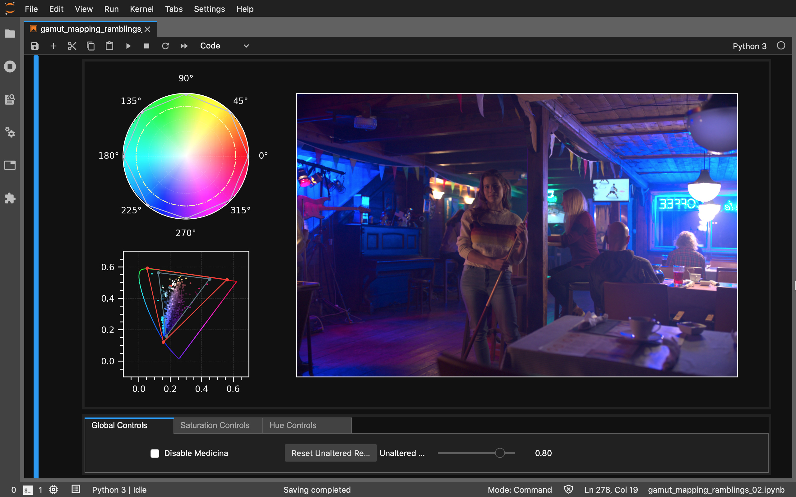
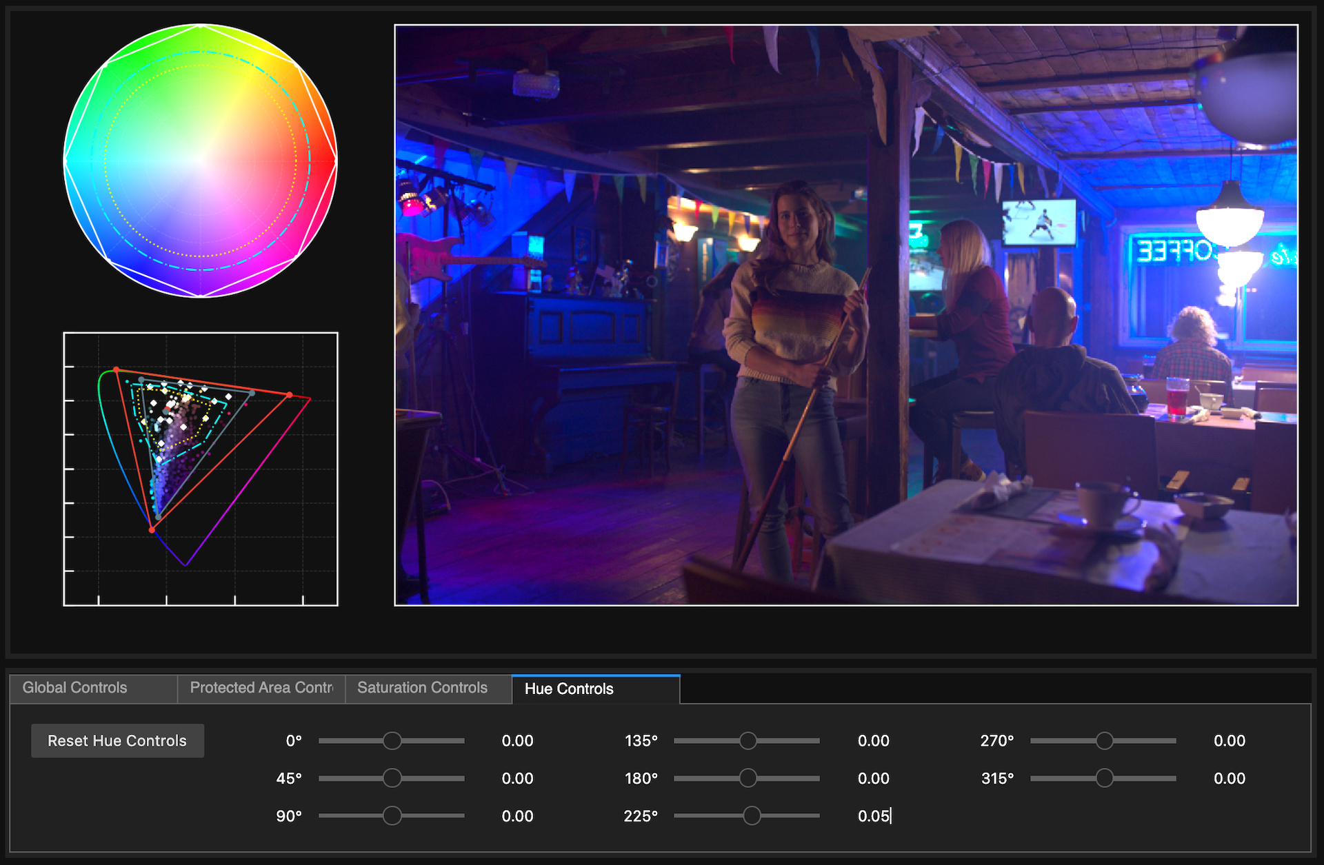
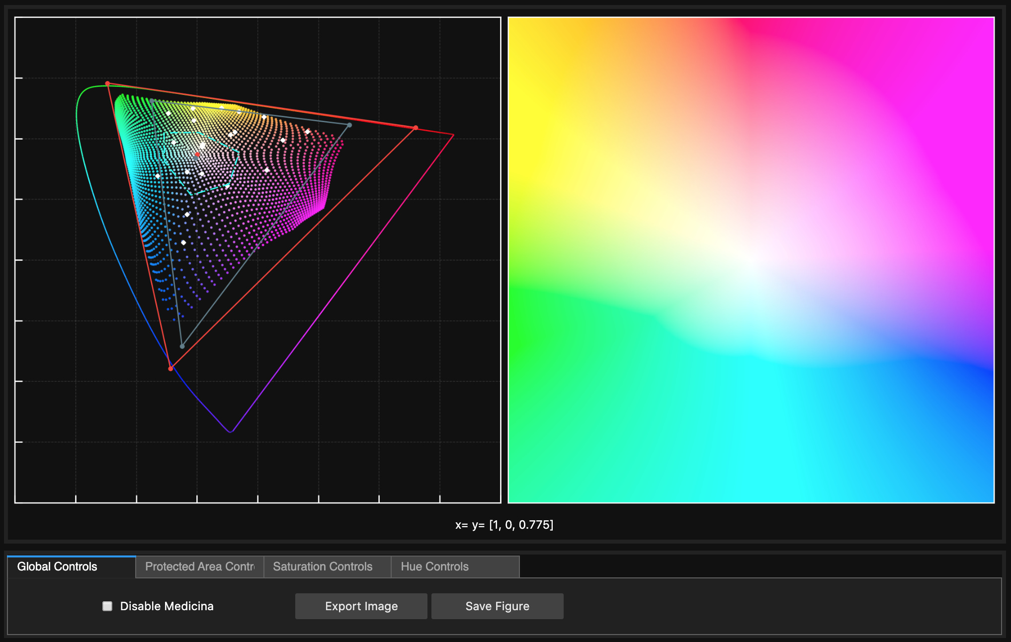
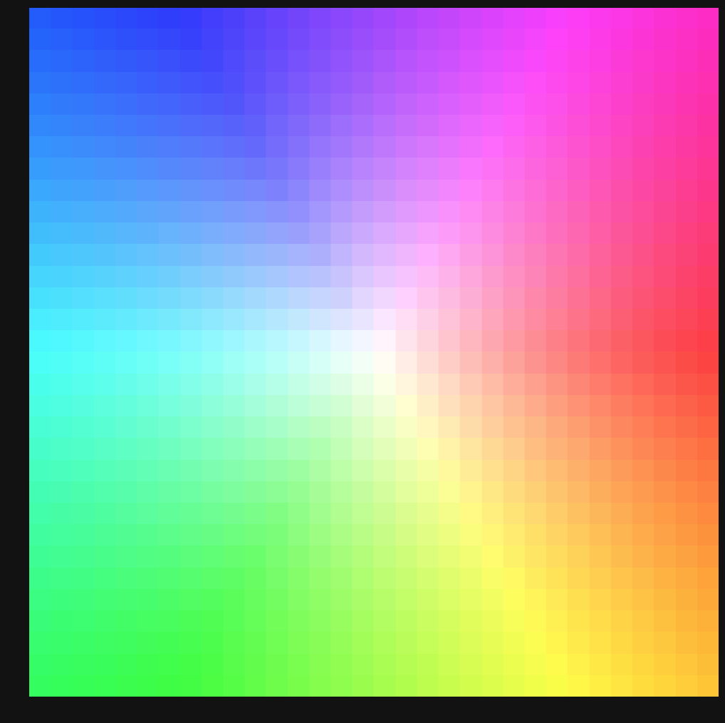
I have been exploring gamut mapping in cylindrical spaces/polar coordinates lately, a few images courtesy @martin.smekal first (note that there is no proper View Transform here, i.e. brut sRGB):
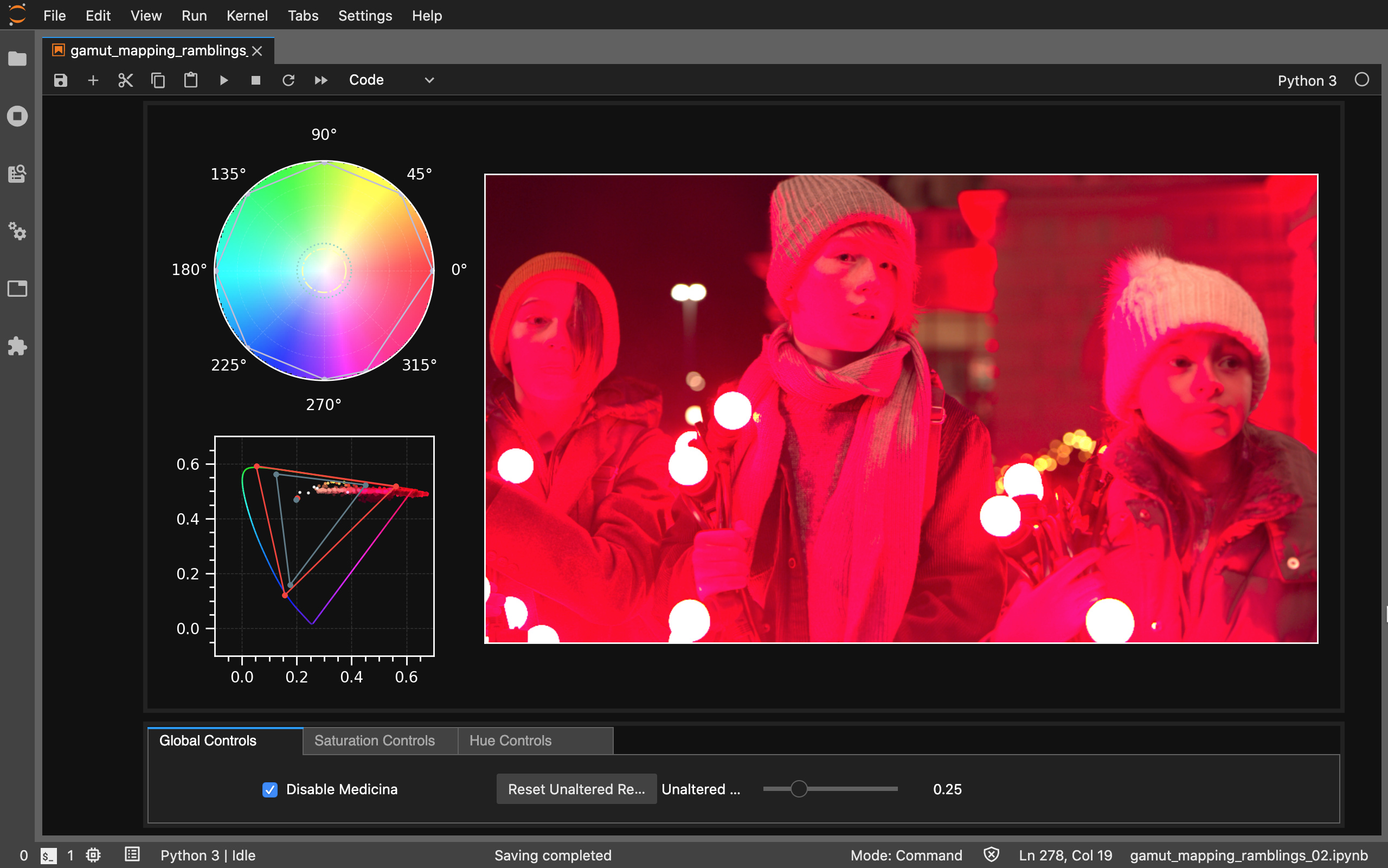
Here, I excessively adjusted the compression threshold and compressed heavily the magenta wedge to fit everything in sRGB.
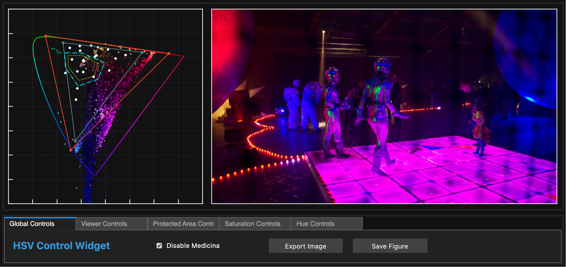
Don’t be fooled by the UI, it is super slow (on my old laptop).
The current model is deceptively simple: HSV with Control over Hue Wedges, Saturation Compression, and Unaltered Region. It is very close to the first model @matthias.scharfenber presented in Nuke (and for good reason, I do use that since a few years in UE4 and Unity). I tried a few cylindrical models that did not much good, e.g. HCL and will give a stab at IHLS.
The current model is (from initial tests and TBC):
Exposure Invariant
Gamut Agnostic
Invertible
Vectorisable
Nothing to play with or share as of now as I’m still exploring (and need to clean up that thing).
Nice, @Thomas_Mansencal! Looking promising. Thanks for the work in making it easy to visualize, too - looking forward to playing with it once you share your magic
Are those test images something we could add to the dropbox? Would be great additions.
Not much magic for now, just basic things! I think that @sdyer sent the upload link to @martin.smekal earlier, so we should get those images at some point.
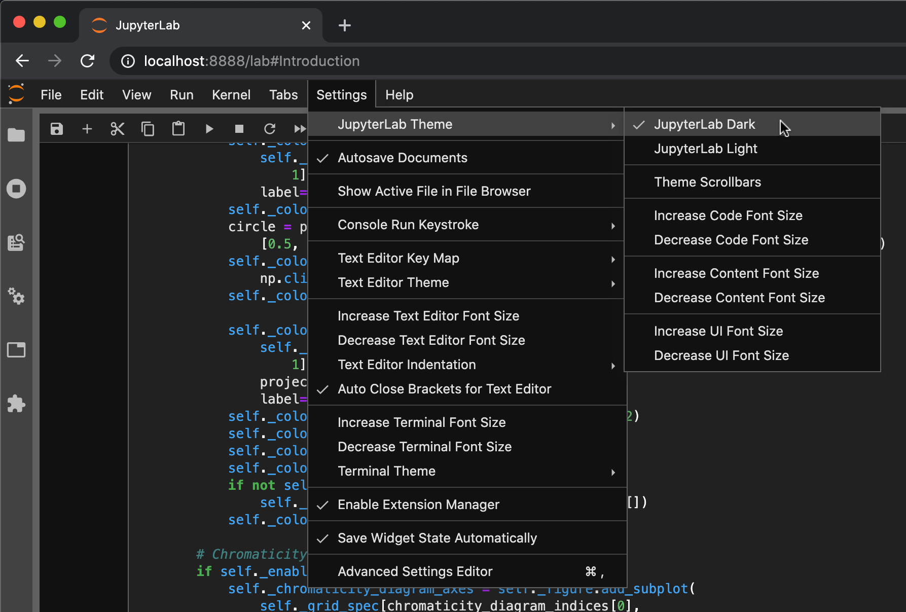
Great work! I tried to install and run this on windows. Apparently Poetry has some problems on windows with installing dependencies so i pip installed them manually. Everything else works but after I run “poetry run jupyter lab” jupyterlab opens but then I just see the github folder with all the files. Where do I go from here or is my installation broken because of my manual pip installation?
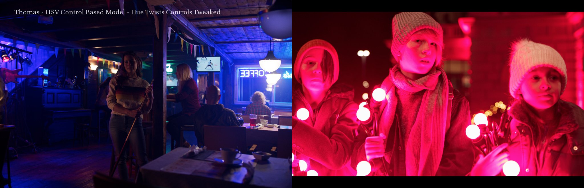
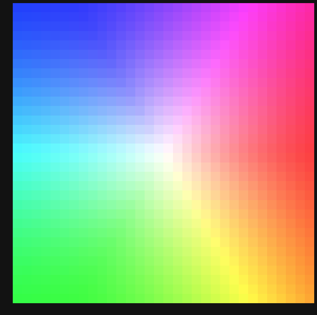
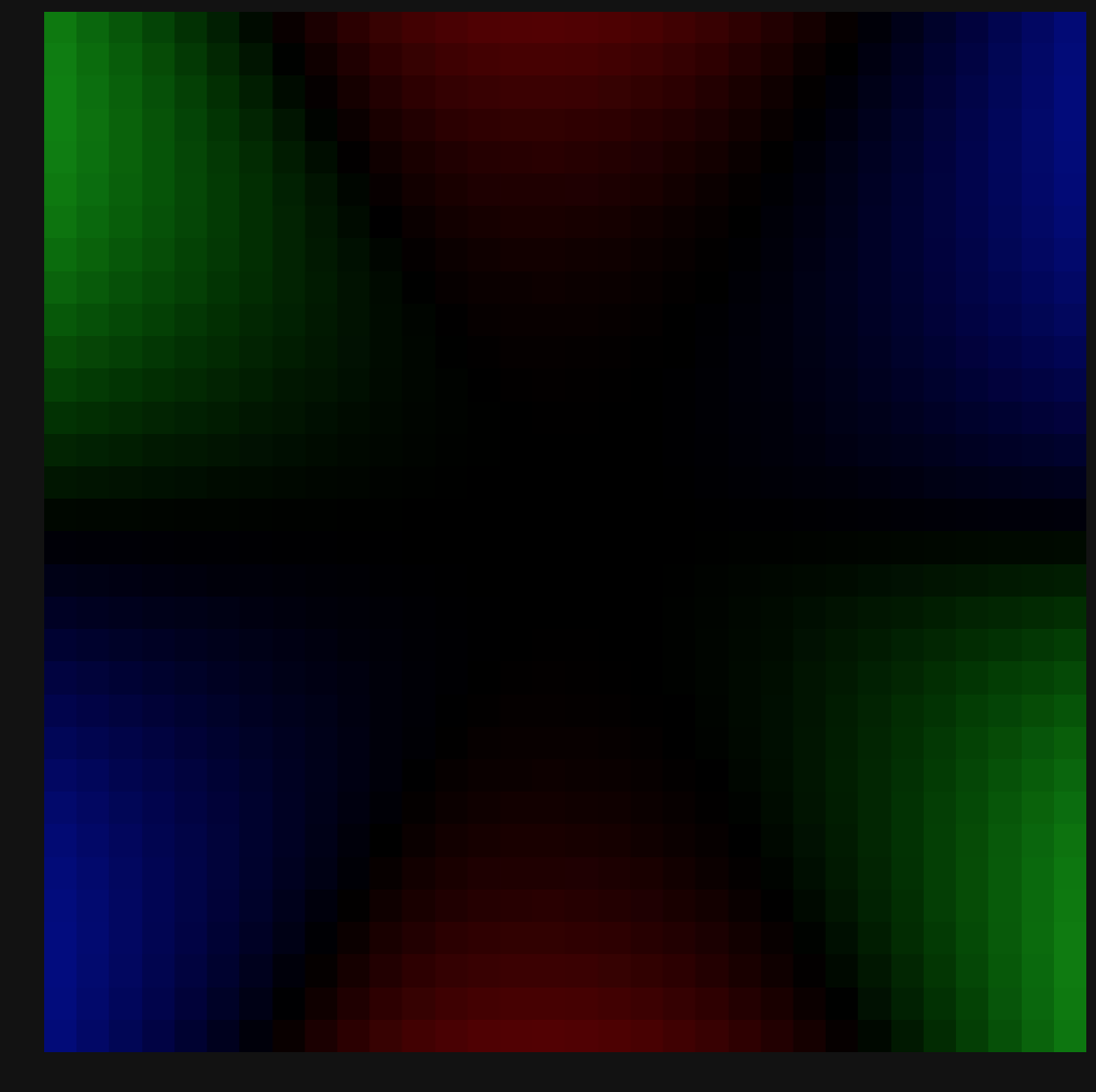
When comparing both the RGB Saturation and HSV Control models I noticed a cyclic pattern in the way they differ: the HSV Control model tends to clump the intermediary colours toward the primary and secondary ones which I assumed could be solved if not entirely, at least partially with the Hue Controls.
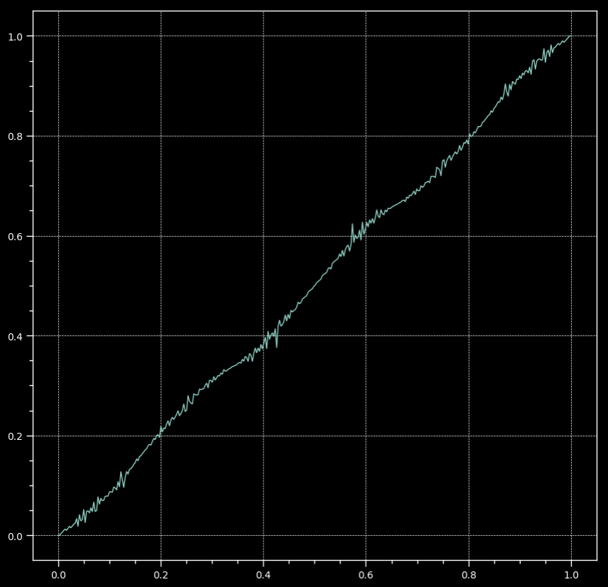
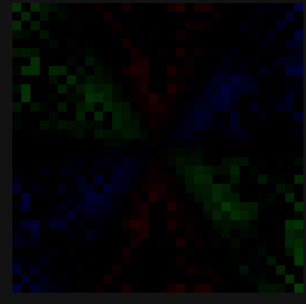
With that in mind, I tried to naively brute force the required Hue Offsets to reduce the error between the two models. Interestingly enough and even though I did not give a chance to the optimisation to finish, here is the resulting Hue Lookup with abscissa representing the Hue Angle and ordinate the Hue Offset:
Quite cool because it confirms my gut feeling that the HSV Control model should be able to achieve results in the ballpark of the RGB Saturation one. I will come up with clean offsets in the coming days. Of interest for you @matthias.scharfenber
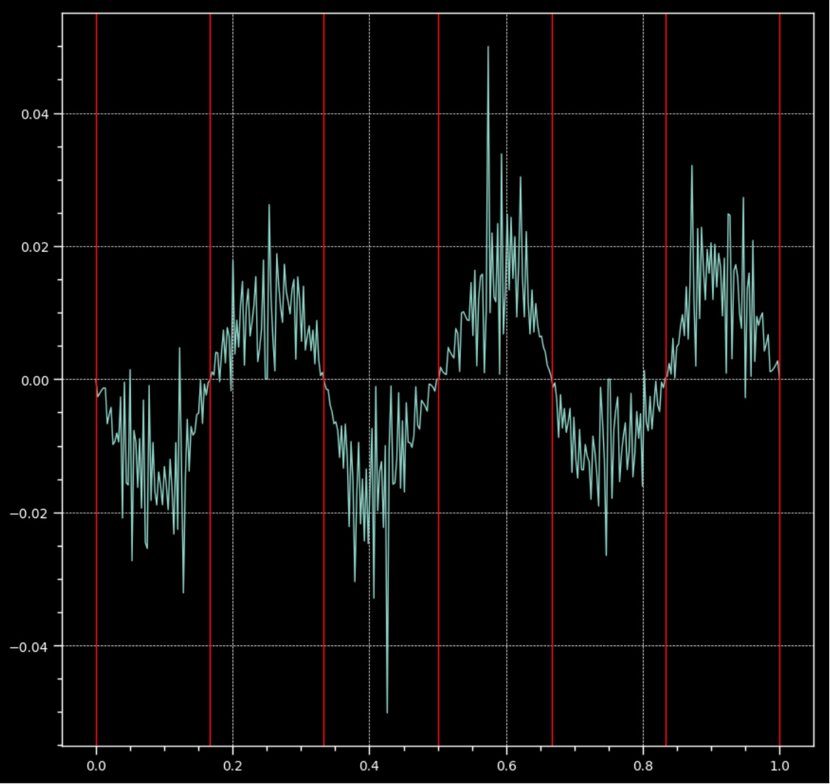
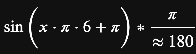
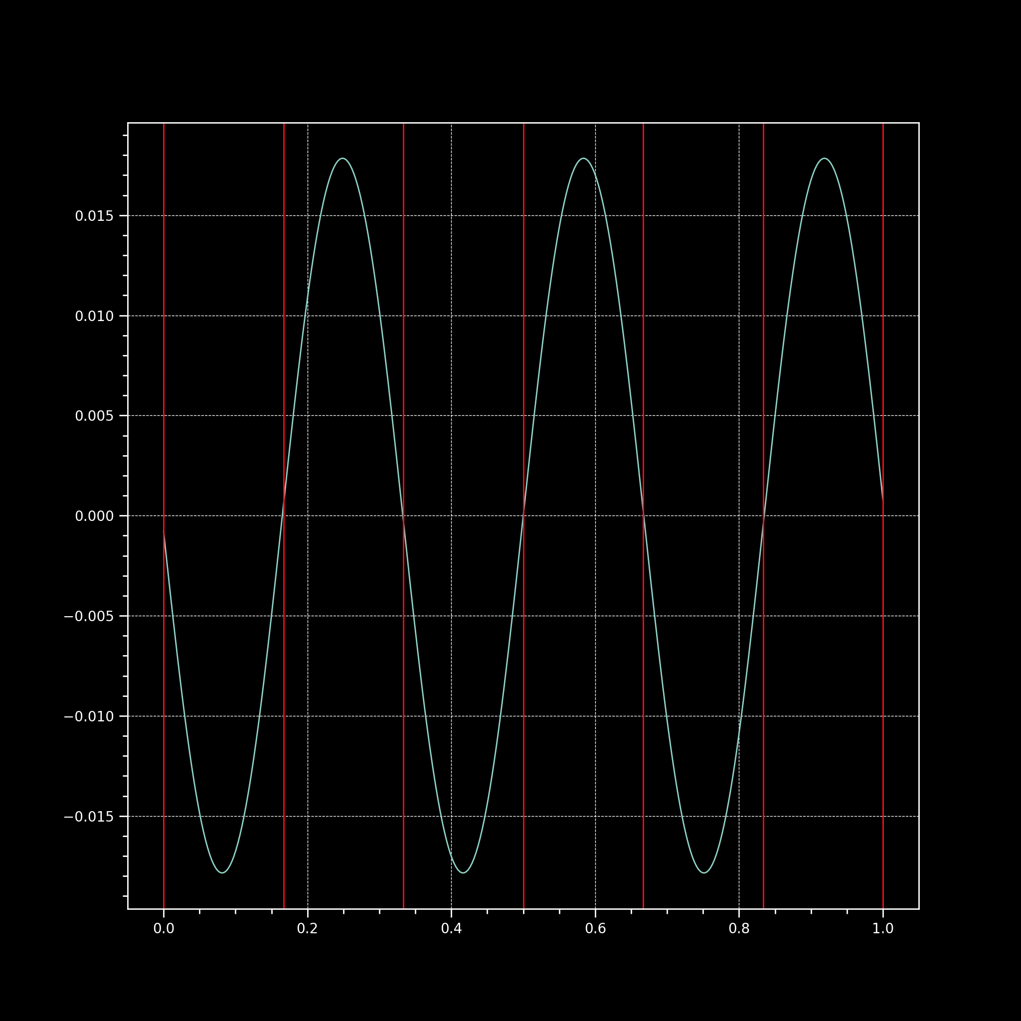
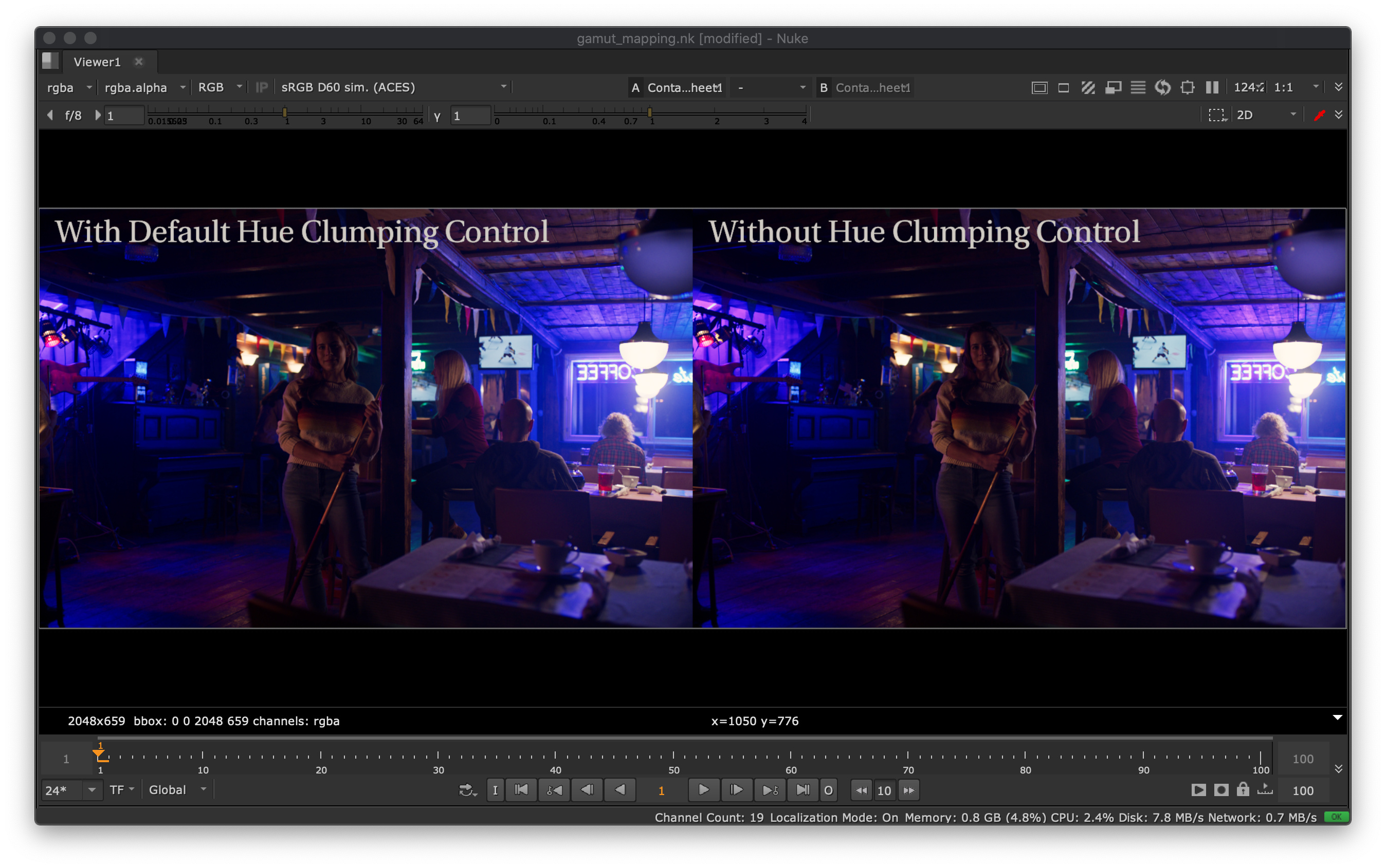
I spent some more time digging tonight and turns out that a very close fitting function is as follows (180 just happened to be a convenient rounded value):
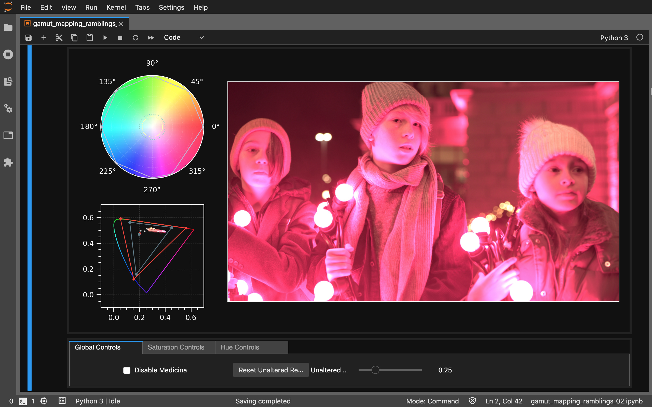
So this almost fixes the dreaded magenta cast plaguing the HSV model while giving some controls over the hue.
Parameterising the 180 constant allows to vary the clumping around the primary and secondary colours. I have not rolled that yet in the Jupyter Notebook but here are some Nuke nodes (that do not have the Hue Twist Controls):
set cut_paste_input [stack 0]
version 12.1 v1
Read {
 inputs 0
 file_type exr
 file /Users/kelsolaar/Documents/Development/colour-science/gamut-mapping-ramblings/resources/images/A009C002_190210_R0EI_Alexa_LogCWideGamut.exr
 format "1024 659 0 0 1024 659 1 "
 origset true
 name Read15
 selected true
 xpos -40
 ypos -114
}
Shuffle2 {
 fromInput1 {{0} B}
 fromInput2 {{0} B}
 mappings "4 rgba.red 0 0 rgba.red 0 0 rgba.green 0 1 rgba.green 0 1 rgba.blue 0 2 rgba.blue 0 2 white -1 -1 rgba.alpha 0 3"
 name Shuffle1
 selected true
 xpos -40
 ypos -33
}
ColorMatrix {
 matrix {
     {1.451439316 -0.2365107469 -0.2149285693}
     {-0.0765537733 1.1762297 -0.0996759265}
     {0.0083161484 -0.0060324498 0.9977163014}
   }
 name ACES2065-1_to_ACEScg
 selected true
 xpos -40
 ypos -9
}
set N27d0e000 [stack 0]
Expression {
 temp_name0 cmax
 temp_expr0 max(r,g,b)
 temp_name1 cmin
 temp_expr1 min(r,g,b)
 temp_name2 delta
 temp_expr2 cmax-cmin
 expr0 delta==0?0:cmax==r?(((g-b)/delta+6)%6)/6:cmax==g?(((b-r)/delta+2)/6):(((r-g)/delta+4)/6)
 expr1 "cmax == 0 ? 0 : delta / cmax"
 expr2 cmax
 name RGB_to_HSV
 note_font "Bitstream Vera Sans"
 selected true
 xpos -40
 ypos 39
}
set N279a9800 [stack 0]
Expression {
 temp_name0 i
 temp_expr0 i_Floating_Point_Slider
 temp_name1 o
 temp_expr1 o_Floating_Point_Slider
 expr0 "clamp((r - i) / (o - i) ** 2 * (3 - 2 * (r - i) / (o - i)))"
 expr1 "clamp((g - i) / (o - i) ** 2 * (3 - 2 * (g - i) / (o - i)))"
 expr2 "clamp((b - i) / (o - i) ** 2 * (3 - 2 * (b - i) / (o - i)))"
 name Smoothstep
 selected true
 xpos -150
 ypos 87
 addUserKnob {20 User}
 addUserKnob {7 i_Floating_Point_Slider l i}
 i_Floating_Point_Slider {0.7}
 addUserKnob {7 o_Floating_Point_Slider l o}
 o_Floating_Point_Slider {{parent.tanh_Compression.t_Floating_Point_Slider}}
}
push $N27d0e000
push $N279a9800
Dot {
 name Dot17
 selected true
 xpos 104
 ypos 42
}
Expression {
 temp_name0 t
 temp_expr0 t_Floating_Point_Slider
 temp_name1 l
 temp_expr1 l_Floating_Point_Slider
 expr0 "r > t ? t + l * tanh((r - t) / l) : r"
 expr1 "g > t ? t + l * tanh((g - t) / l) : g"
 expr2 "b > t ? t + l * tanh((b - t) / l) : b"
 name tanh_Compression
 selected true
 xpos 70
 ypos 87
 addUserKnob {20 User}
 addUserKnob {7 t_Floating_Point_Slider l a}
 t_Floating_Point_Slider 0.8
 addUserKnob {7 l_Floating_Point_Slider l b}
 l_Floating_Point_Slider {{"1 - t_Floating_Point_Slider"}}
}
Dot {
 name Dot18
 selected true
 xpos 104
 ypos 162
}
push $N279a9800
Expression {
 expr0 "r + sin(r*pi*6+pi)*(pi/a_Floating_Point_Slider)"
 expr1 "g + sin(g*pi*6+pi)*(pi/a_Floating_Point_Slider)"
 expr2 "b + sin(b*pi*6+pi)*(pi/a_Floating_Point_Slider)"
 name Clumping_Expression
 selected true
 xpos -40
 ypos 111
 addUserKnob {20 User}
 addUserKnob {7 a_Floating_Point_Slider l a R 90 270}
 a_Floating_Point_Slider 180
}
Expression {
 expr0 "r % 1"
 name Modulus_Expression
 selected true
 xpos -40
 ypos 135
}
ShuffleCopy {
 inputs 2
 green green
 alpha alpha2
 name ShuffleCopy
 note_font "Bitstream Vera Sans"
 selected true
 xpos -40
 ypos 159
}
Expression {
 temp_name0 C
 temp_expr0 b*g
 temp_name1 X
 temp_expr1 C*(1-abs((r*6)%2-1))
 temp_name2 m
 temp_expr2 b-C
 expr0 (r<1/6?C:r<2/6?X:r<3/6?0:r<4/6?0:r<5/6?X:C)+m
 expr1 (r<1/6?X:r<2/6?C:r<3/6?C:r<4/6?X:r<5/6?0:0)+m
 expr2 (r<1/6?0:r<2/6?0:r<3/6?X:r<4/6?C:r<5/6?C:X)+m
 name HSV_to_RGB
 note_font "Bitstream Vera Sans"
 selected true
 xpos -40
 ypos 183
}
Merge2 {
 inputs 2+1
 maskChannelMask rgba.red
 name Merge1
 selected true
 xpos -150
 ypos 183
}
Viewer {
 frame_range 1-100
 viewerProcess "sRGB (ACES)"
 name Viewer1
 selected true
 xpos -150
 ypos 207
}
Gamut volume clipping, at the top and bottom of the gamut volume, resulting in hue skew as the colour ratios end up broken.
Inherent nonlinearity with of the underlying photometric xy model with respect to desaturation approaches, hence implied Abney mixing on any gamut clip along saturation. Any form of additive achromatic light or implied additive achromatic light via a gamut transform and area clip will manifest this problem. It’s somewhat avoiding the discussion of a more “correct” physically plausible desaturation.
But can you have a physically-plausible solution when no model gives paths/space distortion outside the spectral locus, i.e. in the non-physical realm?
For example, what paths the values in that blue lump should be taking?
That’s a very exciting proposition, I’d say? At least worth spending a sliver of time on? At the cursory evidence level, I’d say there is enough compelling evidence to suggest that it is at least plausible!
I think that’s pretty clear, no? More than enough research on that front with a very direct line to the proper path for S cone response, and a good enough of an entry point to seek a solution for L cone.
Sorry, no it is not clear at all! It is the realm of extrapolation/prediction, outside the known human dataset: we don’t have any data for what is outside the spectral locus and for good reason, we cannot see it! If you are asking me what should values do there, well I don’t know
Except we are already carrying forward via extrapolation as it is, using what we believe is reasonable, and it doesn’t seem to be stopping anyone.
With that said, I’d suggest that there is at least as compelling evidence on what should happen within the spectral locus that gives us a much better indication of a decent path forward. (IE Not the Abney approach.)
There’s no difference between extrapolating that theory to the approach and using it to push values into the spectral locus than the current body of equally reasonable assumptions. It would be an equivalent construct of broken at the very worst.
But without any assumptions on the underlying space. Starting to make assumptions is what is dangerous here, especially if we stray away from any linear transformation.
With respect to perceptual attributes, yes, with respect to XYZ itself, the transformation dictates if it is linear or not, likewise for any other space. One point that was talked about very early in the first Working Group meetings is that we cannot really use perceptual attributes for scene-referred transformations because we don’t have a model for that.
Full agreement. They also appear to be rather brittle.
The question is ultimately whether or not it is plausible to work closer to energy conservation and use an alternative means of desaturation other than Abney based.