RGB Saturation Gamut Mapping Approach and a Comp/VFX Perspective

Roll-off start is set with a and limit by b: https://www.desmos.com/calculator/uz0if9qc1h, make b free to set the limit to your wish.

I have made a Resolve DCTL version of @jedsmith’s BlinkScript. This allows it to run in real-time on moving footage.

DCTL_gamut_mapper

5 Likes

That helped me figure it out. Thanks for teaching me math @Thomas_Mansencal :stuck_out_tongue:

I have a few more updates. I figured out the bug with calculating the inverse. It was just a simple thing I missed. I needed to correctly inverse the calculation of the scale factor.

Thanks to Thomas’ help with the tanh function I was able to get the parameters to behave the same between both methods. For the limit controls of cyan, magenta, or yellow: When limit is at 0, no compression is applied. When limit is at 1, out of gamut colors are compressed to the gamut boundary. When limit is greater than 1 (with a max of 1/(1-threshold) which would be a hard clip), out of gamut colors are compressed more than the gamut boundary.

For inverting the gamut compression, there are still differences. I think it is caused by the asymptotic nature of the compression curve and a lack of precision, but it could very well be something else that I’m missing. Anyone sees something I’m not please let me know! :smiley:

I am able to get a perfect roundtrip if I use the original non-gamut compressed image to calculate the achromatic distance from… To allow this workflow I’ve added a “orig” input on the nuke node.

Updated blinkscript and nuke expression node is here:

@nick Thanks for the DCTL! That should be useful. It’s pretty cool how similar CTL and C is, it’s super easy to port C code over.

As before here’s the full source for the blinkscript so it’s easy to look over:

kernel GamutCompression : ImageComputationKernel<ePixelWise> {
  Image<eRead, eAccessPoint, eEdgeClamped> src;
  Image<eWrite> dst;

  param:
    float threshold;
    float cyan;
    float magenta;
    float yellow;
    int method;
    bool invert;
    bool distance;
    bool d_compressed;

  // calc hyperbolic tangent
  float tanh( float in) {
    float e = 2.718281828459f;
    float f = pow(e, 2*in);
    return (f-1.0f) / (f+1.0f);
  }

  // calc inverse hyperbolic tangent
  float atanh( float in) {
    return log((1.0f+in)/(1.0f-in))/2.0f;
  }

  void process() {

    // thr is the complement of threshold. 
    // that is: the percentage of the core gamut to protect
    float thr = 1.0f - threshold;

    // bias limits by color component
    // range is limited to 0.00001 > lim < 1/thr
    // cyan = 0: no compression
    // cyan = 1: "normal" compression with limit at 1.0
    // 1 > cyan < 1/thr : compress more than edge of gamut. max = hard clip (e.g., thr=0.8, max = 1.25)
    float3 lim;
    lim.x = 1.0f/max(0.00001f, min(1.0f/thr, cyan));
    lim.y = 1.0f/max(0.00001f, min(1.0f/thr, magenta));
    lim.z = 1.0f/max(0.00001f, min(1.0f/thr, yellow));

    float r = src().x;
    float g = src().y;
    float b = src().z;

    // achromatic axis 
    float ach = max(r, max(g, b));

    // distance from the achromatic axis for each color component
    float d_r = ach == 0 ? 0 : sqrt( pow(r-ach, 2.0f)) / ach;
    float d_g = ach == 0 ? 0 : sqrt( pow(g-ach, 2.0f)) / ach;
    float d_b = ach == 0 ? 0 : sqrt( pow(b-ach, 2.0f)) / ach;
    

    // compress distance for each color component
    float cd_r, cd_g, cd_b;
    if (method == 0.0f) {
      // hyperbolic tangent softclip method suggested by Thomas Mansencal here
      // https://community.acescentral.com/t/simplistic-gamut-mapping-approaches-in-nuke/2679/2
      // gives good results, but perhaps the curve is too asymptotic. very little color shift.
      // example plot: https://www.desmos.com/calculator/jtvzbae25q
      cd_r = d_r > thr ? thr + (lim.x - thr) * tanh( ( (d_r - thr)/( lim.x-thr))) : d_r;
      cd_g = d_g > thr ? thr + (lim.y - thr) * tanh( ( (d_g - thr)/( lim.y-thr))) : d_g;
      cd_b = d_b > thr ? thr + (lim.z - thr) * tanh( ( (d_b - thr)/( lim.z-thr))) : d_b;

      if (invert == 1.0f) {
          cd_r = d_r > thr ? thr + (lim.x - thr) * atanh( d_r/( lim.x - thr) - thr/( lim.x - thr)) : d_r;
          cd_g = d_g > thr ? thr + (lim.y - thr) * atanh( d_g/( lim.y - thr) - thr/( lim.y - thr)) : d_g;
          cd_b = d_b > thr ? thr + (lim.z - thr) * atanh( d_b/( lim.z - thr) - thr/( lim.z - thr)) : d_b;
      }
    } else if (method == 1.0f) {
      // softclip method suggested by Nick Shaw here
      // https://community.acescentral.com/t/simplistic-gamut-mapping-approaches-in-nuke/2679/3
      // good results, easy to bias look with limits
      // example plot: https://www.desmos.com/calculator/jyewfptd4y
      cd_r = d_r > thr ? thr+(-1/((d_r-thr)/(lim.x-thr)+1)+1)*(lim.x-thr) : d_r;
      cd_g = d_g > thr ? thr+(-1/((d_g-thr)/(lim.y-thr)+1)+1)*(lim.y-thr) : d_g;
      cd_b = d_b > thr ? thr+(-1/((d_b-thr)/(lim.z-thr)+1)+1)*(lim.z-thr) : d_b;

      if (invert == 1.0f) {
        // inversed compression distance for each color component
        cd_r = d_r > thr ? (pow(thr, 2.0f) - thr*d_r + (lim.x-thr)*d_r) / (thr + (lim.x-thr) - d_r) : d_r;
        cd_g = d_g > thr ? (pow(thr, 2.0f) - thr*d_g + (lim.y-thr)*d_g) / (thr + (lim.y-thr) - d_g) : d_g;
        cd_b = d_b > thr ? (pow(thr, 2.0f) - thr*d_b + (lim.z-thr)*d_b) / (thr + (lim.z-thr) - d_b) : d_b;
      }
    }

    float c_r, c_g, c_b;
    if (invert == 1.0f) {
      // scale up each color component relative to achromatic axis by gamut uncompression factor
      c_r = (r-ach)*((cd_r-d_r)+1.0f)+ach;
      c_g = (g-ach)*((cd_g-d_g)+1.0f)+ach;
      c_b = (b-ach)*((cd_b-d_b)+1.0f)+ach;

    } else {
      // scale down each color component relative to achromatic axis by gamut compression factor
      c_r = (r-ach)/((d_r-cd_r)+1.0f)+ach;
      c_g = (g-ach)/((d_g-cd_g)+1.0f)+ach;
      c_b = (b-ach)/((d_b-cd_b)+1.0f)+ach;
    }

    // write to output
    dst() = float4(c_r, c_g, c_b, 1);

    // debug outputs
    if (distance == 1.0f) {
      if (d_compressed == 1.0f) {
        dst() = float4(cd_r, cd_g, cd_b, 1.0f);
      } else {
        dst() = float4(d_r, d_g, d_b, 1.0f);
      }
    }
  }
};
2 Likes

That works very well! Better out-of-the-box than everything I have been musing with so far (I get very similar output by tweaking parameterisation but not as a default), really like how simple and elegant this is. :smiling_face_with_three_hearts:

Cheers,

Thomas

2 Likes

Yeah Jed, this is great work! Will message you about talking through some of the details at a future meeting soon.

Ran Jed’s Model through the two images I’m using currently to do my tests:

Jed’s RGB Saturation Based Model - Threshold 0.15

Thomas’s HSV Control Based Model - Threshold & Hue Twist Controls Tweaked

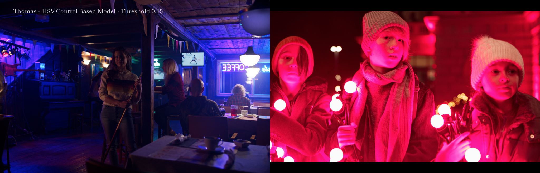
Thomas’s HSV Control Based Model - Threshold 0.15
Note that with default parameters, the model is almost the same than the HSV model of @matthias.scharfenber.

I can get close to Jed’s with mine using the Hue Twists and fiddling a bit with the Threshold but Jed’s default to a much more pleasing output, i.e. less magenta, the Model is simpler, more elegant, faster and easier to implement.

Cheers,

Thomas

The magenta feels like the other half of the missing gamut map, no? Any idea on whether the values are escaping the gamut volume there?

I had planned to update my DCTL implementation to match @jedsmith’s latest BlinkScript. But he has very kindly already done that in his own fork, and submitted a pull request, which I have just merged. Everybody who is testing it should grab the latest version.

2 Likes

from my experience, Jed’s method (I will call it Kirk method :slight_smile: ) works good for scene-referred data for a general any gamut to any gamut mapper, and it ticks all the boxes we have defined :-).

2 Likes

@daniele: I wanted to ask you how close it is from the Filmlight one, seemed quite similar in principle to what you presented a few weeks ago.

It is a pretty similar approach, yes.

1 Like

I was playing around with different tone-mapping algorithms to use for compression of the distance, and came up with a new one based on a natural exponent function. It is between the hyperbolic tangent function and the Reinhard style simple tone-mapping function in terms of the aggressiveness of its slope. I think the results are pretty good.

Here’s a plot comparing all three compression functions: https://www.desmos.com/calculator/x69iyptspq

And here’s a few screenshots comparing the three methods


As before, here are the

and source code

kernel GamutCompression : ImageComputationKernel<ePixelWise> {
  Image<eRead, eAccessPoint, eEdgeClamped> src;
  Image<eWrite> dst;

  param:
    float threshold;
    float cyan;
    float magenta;
    float yellow;
    int method;
    bool invert;
    bool distance;
    bool d_compressed;

  // calc hyperbolic tangent
  float tanh( float in) {
    float e = 2.718281828459f;
    float f = pow(e, 2*in);
    return (f-1.0f) / (f+1.0f);
  }

  // calc inverse hyperbolic tangent
  float atanh( float in) {
    return log((1.0f+in)/(1.0f-in))/2.0f;
  }

  void process() {

    // thr is the complement of threshold. 
    // that is: the percentage of the core gamut to protect
    float thr = 1.0f - threshold;

    // bias limits by color component
    // range is limited to 0.00001 > lim < 1/thr
    // cyan = 0: no compression
    // cyan = 1: "normal" compression with limit at 1.0
    // 1 > cyan < 1/thr : compress more than edge of gamut. max = hard clip (e.g., thr=0.8, max = 1.25)
    float3 lim;
    lim.x = 1.0f/max(0.00001f, min(1.0f/thr, cyan));
    lim.y = 1.0f/max(0.00001f, min(1.0f/thr, magenta));
    lim.z = 1.0f/max(0.00001f, min(1.0f/thr, yellow));

    float r = src().x;
    float g = src().y;
    float b = src().z;

    // achromatic axis 
    float ach = max(r, max(g, b));

    // distance from the achromatic axis for each color component
    float d_r = ach == 0 ? 0 : sqrt( pow(r-ach, 2.0f)) / ach;
    float d_g = ach == 0 ? 0 : sqrt( pow(g-ach, 2.0f)) / ach;
    float d_b = ach == 0 ? 0 : sqrt( pow(b-ach, 2.0f)) / ach;
    

    // compress distance for each color component
    float cd_r, cd_g, cd_b;
    if (method == 0.0f) {
      // hyperbolic tangent softclip method suggested by Thomas Mansencal here
      // https://community.acescentral.com/t/simplistic-gamut-mapping-approaches-in-nuke/2679/2
      // gives good results, but perhaps the curve is too asymptotic. very little color shift.
      // example plot: https://www.desmos.com/calculator/jtvzbae25q
      cd_r = d_r > thr ? thr + (lim.x - thr) * tanh( ( (d_r - thr)/( lim.x-thr))) : d_r;
      cd_g = d_g > thr ? thr + (lim.y - thr) * tanh( ( (d_g - thr)/( lim.y-thr))) : d_g;
      cd_b = d_b > thr ? thr + (lim.z - thr) * tanh( ( (d_b - thr)/( lim.z-thr))) : d_b;

      if (invert == 1.0f) {
          cd_r = d_r > thr ? thr + (lim.x - thr) * atanh( d_r/( lim.x - thr) - thr/( lim.x - thr)) : d_r;
          cd_g = d_g > thr ? thr + (lim.y - thr) * atanh( d_g/( lim.y - thr) - thr/( lim.y - thr)) : d_g;
          cd_b = d_b > thr ? thr + (lim.z - thr) * atanh( d_b/( lim.z - thr) - thr/( lim.z - thr)) : d_b;
      }
    } else if (method == 1.0f) {
      // softclip method suggested by Nick Shaw here
      // https://community.acescentral.com/t/simplistic-gamut-mapping-approaches-in-nuke/2679/3
      // good results, easy to bias look with limits
      // example plot: https://www.desmos.com/calculator/jyewfptd4y
      cd_r = d_r > thr ? thr+(-1/((d_r-thr)/(lim.x-thr)+1)+1)*(lim.x-thr) : d_r;
      cd_g = d_g > thr ? thr+(-1/((d_g-thr)/(lim.y-thr)+1)+1)*(lim.y-thr) : d_g;
      cd_b = d_b > thr ? thr+(-1/((d_b-thr)/(lim.z-thr)+1)+1)*(lim.z-thr) : d_b;

      if (invert == 1.0f) {
        // inversed compression distance for each color component
        cd_r = d_r > thr ? (pow(thr, 2.0f) - thr*d_r + (lim.x-thr)*d_r) / (thr + (lim.x-thr) - d_r) : d_r;
        cd_g = d_g > thr ? (pow(thr, 2.0f) - thr*d_g + (lim.y-thr)*d_g) / (thr + (lim.y-thr) - d_g) : d_g;
        cd_b = d_b > thr ? (pow(thr, 2.0f) - thr*d_b + (lim.z-thr)*d_b) / (thr + (lim.z-thr) - d_b) : d_b;
      }
    }

    float c_r, c_g, c_b;
    if (invert == 1.0f) {
      // scale up each color component relative to achromatic axis by gamut uncompression factor
      c_r = (r-ach)*((cd_r-d_r)+1.0f)+ach;
      c_g = (g-ach)*((cd_g-d_g)+1.0f)+ach;
      c_b = (b-ach)*((cd_b-d_b)+1.0f)+ach;

    } else {
      // scale down each color component relative to achromatic axis by gamut compression factor
      c_r = (r-ach)/((d_r-cd_r)+1.0f)+ach;
      c_g = (g-ach)/((d_g-cd_g)+1.0f)+ach;
      c_b = (b-ach)/((d_b-cd_b)+1.0f)+ach;
    }

    // write to output
    dst() = float4(c_r, c_g, c_b, 1);

    // debug outputs
    if (distance == 1.0f) {
      if (d_compressed == 1.0f) {
        dst() = float4(cd_r, cd_g, cd_b, 1.0f);
      } else {
        dst() = float4(d_r, d_g, d_b, 1.0f);
      }
    }
  }
};
2 Likes

Hi @jedsmith,

Something you will find is that the derivatives of all those functions (besides tanh) are not smooth which means that there is a kink at the graft point, it is probably not visible but it is important to be aware of. I added them to your Desmos example: https://www.desmos.com/calculator/bt901oznbm

Cheers,

Thomas

PS: This goes without saying that I favour smooth derivatives! :slight_smile:

Curious what specific portion of the chain is causing this posterization error:

@Troy_James_Sobotka it looks like this is caused by brightening of the out of gamut areas of the face, which have less noise from the camera sensor. I made a little screencapture and uploaded it in a terribly compressed gif with lots of posterization … hopefully it gets the idea across anyway :stuck_out_tongue:

This one is with the tanh curve
face_gamut_compress_tanh

This one is with the “simple” curve.
face_gamut_compress_simple

Interestingly, the “simple” compression method with a limit of around 0.8 has less of this visual artifact.

With the much more aggressive slope of the “simple” curve and limiting it to 0.8, it brings the question: how far outside of gamut do we need to go when compressing values in? And if it’s not to infinity, what compression curve has the least visual artifacts? This is something I think we need to figure out.

1 Like

Another update:
I have fixed the invertibility issues.

I realized after an embarrassingly long time that c_r could be defined completely in terms of ach and cd_r (achromatic and compressed distance, respectively). This allows the gamut compression to be exactly inverted.

As before:

kernel GamutCompression : ImageComputationKernel<ePixelWise> {
  Image<eRead, eAccessPoint, eEdgeClamped> src;
  Image<eWrite> dst;

  param:
    float threshold;
    float cyan;
    float magenta;
    float yellow;
    int method;
    bool invert;

  // calc hyperbolic tangent
  float tanh( float in) {
    float f = exp(2.0f*in);
    return (f-1.0f) / (f+1.0f);
  }

  // calc inverse hyperbolic tangent
  float atanh( float in) {
    return log((1.0f+in)/(1.0f-in))/2.0f;
  }

  void process() {
    // thr is the complement of threshold. 
    // that is: the percentage of the core gamut to protect
    float thr = 1.0f - threshold;

    // bias limits by color component
    // range is limited to 0.00001 > lim < 1/thr
    // cyan = 0: no compression
    // cyan = 1: "normal" compression with limit at 1.0
    // 1 > cyan < 1/thr : compress more than edge of gamut. max = hard clip (e.g., thr=0.8, max = 1.25)
    float3 lim;
    lim.x = 1.0f/max(0.00001f, min(1.0f/thr, cyan));
    lim.y = 1.0f/max(0.00001f, min(1.0f/thr, magenta));
    lim.z = 1.0f/max(0.00001f, min(1.0f/thr, yellow));

    float r = src().x;
    float g = src().y;
    float b = src().z;

    // achromatic axis 
    float ach = max(r, max(g, b));

    // distance from the achromatic axis for each color component
    float d_r, d_g, d_b;
    d_r = ach == 0 ? 0 : fabs(float(r-ach)) / ach;
    d_g = ach == 0 ? 0 : fabs(float(g-ach)) / ach;
    d_b = ach == 0 ? 0 : fabs(float(b-ach)) / ach;

    // compress distance for each color component
    // method 0 : tanh - hyperbolic tangent compression method suggested by Thomas Mansencal https://community.acescentral.com/t/simplistic-gamut-mapping-approaches-in-nuke/2679/2
    // method 1 : exp - natural exponent compression method
    // method 2 : simple - simple Reinhard type compression suggested by Nick Shaw https://community.acescentral.com/t/simplistic-gamut-mapping-approaches-in-nuke/2679/3
    // example plots for each method: https://www.desmos.com/calculator/x69iyptspq
    float cd_r, cd_g, cd_b;
    if (method == 0.0f) {
      if (invert == 0.0f) {
        cd_r = d_r > thr ? thr + (lim.x - thr) * tanh( ( (d_r - thr)/( lim.x-thr))) : d_r;
        cd_g = d_g > thr ? thr + (lim.y - thr) * tanh( ( (d_g - thr)/( lim.y-thr))) : d_g;
        cd_b = d_b > thr ? thr + (lim.z - thr) * tanh( ( (d_b - thr)/( lim.z-thr))) : d_b;
      } else {
          cd_r = d_r > thr ? thr + (lim.x - thr) * atanh( d_r/( lim.x - thr) - thr/( lim.x - thr)) : d_r;
          cd_g = d_g > thr ? thr + (lim.y - thr) * atanh( d_g/( lim.y - thr) - thr/( lim.y - thr)) : d_g;
          cd_b = d_b > thr ? thr + (lim.z - thr) * atanh( d_b/( lim.z - thr) - thr/( lim.z - thr)) : d_b;
      }
    } else if (method == 1.0f) {
      if (invert == 0.0f) {
        cd_r = d_r > thr ? lim.x-(lim.x-thr)*exp(-(((d_r-thr)*((1.0f*lim.x)/(lim.x-thr))/lim.x))) : d_r;
        cd_g = d_g > thr ? lim.y-(lim.y-thr)*exp(-(((d_g-thr)*((1.0f*lim.y)/(lim.y-thr))/lim.y))) : d_g;
        cd_b = d_b > thr ? lim.z-(lim.z-thr)*exp(-(((d_b-thr)*((1.0f*lim.z)/(lim.z-thr))/lim.z))) : d_b;
      } else {
        cd_r = d_r > thr ? -log( (d_r-lim.x)/(thr-lim.x))*(-thr+lim.x)/1.0f+thr : d_r;
        cd_g = d_g > thr ? -log( (d_g-lim.y)/(thr-lim.y))*(-thr+lim.y)/1.0f+thr : d_g;
        cd_b = d_b > thr ? -log( (d_b-lim.z)/(thr-lim.z))*(-thr+lim.z)/1.0f+thr : d_b;
      }
    } else if (method == 2.0f) {
      if (invert == 0.0f) {
        cd_r = d_r > thr ? thr+(-1/((d_r-thr)/(lim.x-thr)+1)+1)*(lim.x-thr) : d_r;
        cd_g = d_g > thr ? thr+(-1/((d_g-thr)/(lim.y-thr)+1)+1)*(lim.y-thr) : d_g;
        cd_b = d_b > thr ? thr+(-1/((d_b-thr)/(lim.z-thr)+1)+1)*(lim.z-thr) : d_b;
      } else {
        cd_r = d_r > thr ? (pow(thr, 2.0f) - thr*d_r + (lim.x-thr)*d_r) / (thr + (lim.x-thr) - d_r) : d_r;
        cd_g = d_g > thr ? (pow(thr, 2.0f) - thr*d_g + (lim.y-thr)*d_g) / (thr + (lim.y-thr) - d_g) : d_g;
        cd_b = d_b > thr ? (pow(thr, 2.0f) - thr*d_b + (lim.z-thr)*d_b) / (thr + (lim.z-thr) - d_b) : d_b;
      }
    }

    // scale each color component relative to achromatic axis by gamut compression factor
    float c_r, c_g, c_b;
    c_r = ach-cd_r*ach;
    c_g = ach-cd_g*ach;
    c_b = ach-cd_b*ach;

    // write to output
    dst() = float4(c_r, c_g, c_b, 1);

  }
};

Similarly important is that the derivative does not go flat too early, this not only makes inversion harder but often causes flat image areas.

You were meant to sau flat for too long right? If it is not flat here, it is simply not continuous.

The DCTL is updated again, thanks to a Pull Request from @jedsmith. And I have pushed a couple more commits to ensure the code runs under CUDA, Metal and OpenCL.

2 Likes

I mean that you can see that the derivation of the hyperbolic function reaches 0.0 much earlier than the others. That means many input values get mapped closer together much earlier.