In Part 2, the process for creating empirical LMTs was described. However, empirical LMTs can have limitations that analytic LMTs enable users to avoid.
This post will continue to step through the creation of a LMTs at increasing levels of complexity.
[Transforms used in this article are again provided as CTL code at the end of the article.]
Analytic LMTs
Analytic LMTs are defined mathematically and are expressed as a set of ordered mathematical operations on color component values. The operations can range from simple and concise to as complex as necessary to create a desired look.
The most basic operations are primary color corrections that affect all pixels equally, such as contrast, saturation, and exposure. More complex LMTs might introduce secondary corrections such as hue, saturation, luminance, or a combination of these. Because LMTs are image-wide adjustments, spatial corrections (e.g. windows, garbage mattes, etc.) as well as temporally-variable adjustments (e.g. keyframing) are not currently supported.
A simple example of an analytic LMT is one that applies an ASC CDL as a primary grade. A more complex analytic LMT might adjust saturation based on luminance, qualified by certain hue angles. Even more complex LMTs might chain multiple primary and secondary corrections together. There is no limit to the order of or number of operations allowed in an LMT. There is also no limit imposed on the number of individual LMTs that may be sequenced. It is acceptable (and equivalent) to sequence multiple simple LMTs or to sequence multiple operations within a single LMT file.
Analytic LMT – Example 1 (lower contrast & saturation)
This first example is a simple analytic LMT that adjusts image contrast and saturation. Such a transform could be useful to those who prefer to begin color grading with a lower contrast and saturation than the default in ACES-based projects.
Design approach
Instinctually, it seems the transform should convert ACES2065-1 to ACEScct, apply some ASC CDL-like adjustments, and convert ACEScct back to ACES2065-1 (Figure 4).
The math for each of these individual steps is well defined so writing the code for the full Look Transform is a simple matter of sequencing the individual functions together in order. The ASC CDL parameters can be tuned to the desired level of adjustment.
An alternate design approach
ACEScc or ACEScct are appropriate color spaces in which to apply ASC CDL operations. However, note that there are no rules in the creation or application of LMTs that restrict image contrast adjustment via other operators or in other color spaces. For example, mathematical relationships between linear and log spaces imply that one could instead apply a gamma adjustment in linear space (Figure 5) and attain a similar adjustment to the image contrast as having done a contrast adjustment in a log space.
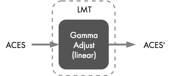 Figure 5. An alternate design approach for an analytic LMT that adjusts image contrast. ACES2065-1 is treated as the “working space” and, because the data is linear, a simple gamma is used to affect contrast.
To demonstrate, an alternate LMT (1c) is also provided that adjusts contrast in linear space using a gamma. This “gamma adjust” transform takes as input both a gamma value and a “pivot” point, which is the linear value around which the slope of that the line will pivot in log-log space. In other words, the pivot defines an anchor point which is “pinned” and will not be modified. The default for this pivot point is set to mid-gray, or an ACES value of 0.18.
Tuning
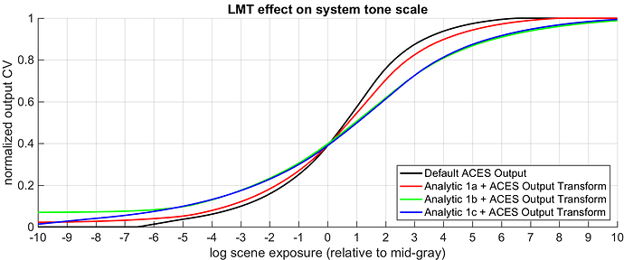
To assist with visualizing the effect of the LMT parameters and tuning the settings, one can utilize a neutral gradient spanning a range of stops centered around mid-gray (ACES=0.18). By plotting exposure level vs. output code value for an ACES Output Transform with no LMT and then overplotting code values from the tuned LMTs + the Output Transform, the effect of the parameters can be compared against the unmodified transform (Figure 6).
On the graph, equal mid-gray levels are indicated if the curves intersect each other at 0 on the scene exposure (relative to mid-gray) axis. In order to keep mid-gray at the same place in the LMT that applies ASC CDL in ACEScct (1a), the offset and power parameters were used to move mid-gray back near its original output level after the slope parameter had been adjusted to decrease contrast. The second LMT that applies ASC CDL in ACEScct (1b) was adjusted to have a contrast even lower than that of LMT 1a, with offset and power again used to restore mid-gray to its pre-slope-adjusted value.
The saturation of images is already somewhat naturally reduced by a decrease in contrast of the tone scales. However, the saturation levels in both 1a and 1b were explicitly further reduced using the ASC CDL “sat” operator.
Analytic LMT 1c uses the alternate approach of adjusting gamma in linear ACES space. The gamma was set to 0.6, which matches the contrast of LMT 1b closely. Note, however, that the curve continues to extend to 0 and doesn’t flare up as it does when contrast is adjusted in ACEScct.
Results
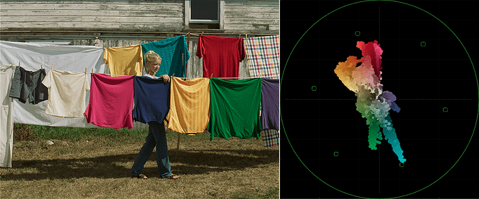
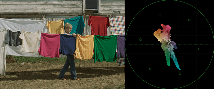
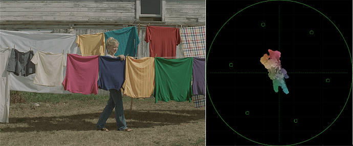
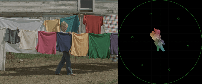
Below you can see the results of the Analytic LMTs on actual images and vector scope plots.
Analytic LMT – Example 2
In Example 1, ASC CDL was used to generically lower image contrast and saturation – a simple process. For most who want a less “contrasty” or “poppy” starting point, this is probably sufficient. But what if one wants to exactly match the neutral tone scale rendering of another transform?
For example, imagine a colorist really likes starting with the “LUT X” look because they are very used to the starting contrast and degree of highlight and shadow rolloff. They want to see exactly the same neutral tone scale rendering on their ACES-based project. Using the process discussed earlier, one could create an empirical LMT to exactly match the “LUT X” look. However, it has already been demonstrated that empirical LMTs have limits. But what if the colorist is really just attached to the tone curve contrast and isn’t necessarily tied to the particular rendering of the colors? This is a perfect case to create an LMT where the neutral tonescale is analyzed and matched, while allowing colors to fall where they will.
Design approach
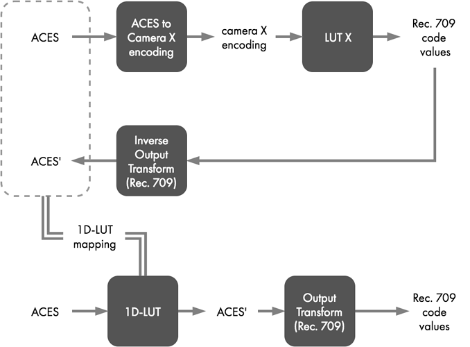
The derivation of a neutral tone scale adjustment required to match the tone curve of “LUT X” is actually quite similar to the procedure used for building empirical LMTs. However, instead of constructing a 3D-LUT, only a 1D-LUT is sought to define the neutral tone scale adjustment that is required such that when ACES2065-1 data is sent through the ACES system tone scale, the net result matches that of LUTX. The appropriate Inverse Output Transform is used to derive the relationship between ACES and ACES’, indicated by the dashed gray box below.
Using an inverse Input Transform, a carefully sampled range of neutral ACES values is converted to the Camera X encoding needed for input to LUT X and then processed through LUT X to get Rec. 709 code values. Those code values are then processed through the Inverse Output Transform for Rec. 709 (combined Inverse Rec. 709 ODT and Inverse RRT), yielding a set of ACES’ values that encapsulate a mapping that will match the neutral tone scale appearance of LUT X through the forward ACES Output Transform. This relationship of input to output, illustrated with a dashed gray box in Figure 11, is derived once and used to populate a 1D-LUT that can drop into an ACES workflow as an LMT to recreate the look of LUT X.
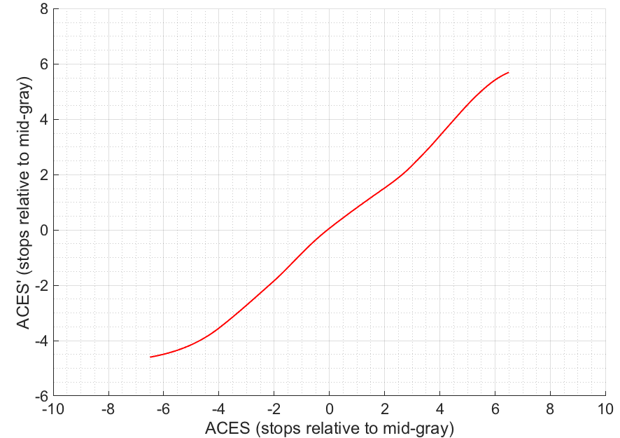
Following the procedure in Figure 11 using a ramp of ACES values logarithmically spaced between -6.5 and +6.5 stops around mid-gray (these points correspond to code values of 0 and 1 on output) results in the 1D-LUT relationship depicted in Figure 12.
However, this 1D-LUT will have the same issue as empirical LUTs and be limited to the output range of the transforms used to derive it. In this specific example, any ACES values above 16.292 will be limited to 9.378, and any ACES values below 0.00198 will be limited to 0.00743. Those are the minimum and maximum linear ACES values that could possibly result through this LMT – only a 10 stop range!
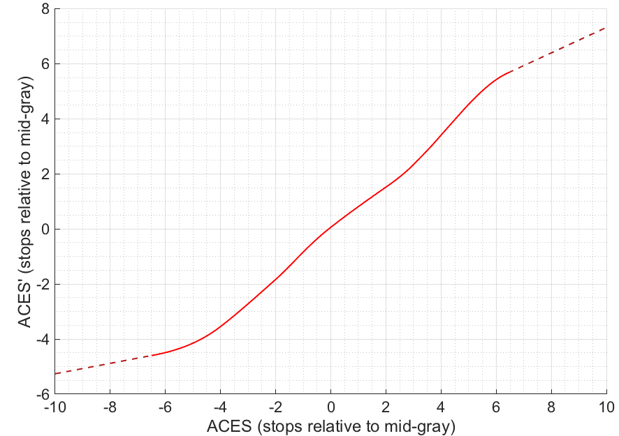
In order to extend the usable range of this 1D-LUT so that images passed through it are not necessarily clamped to that range, one can extrapolate the LUT in log space. By using linear extrapolation in log-log space, a larger range can be supported by the LUT (Figure 13). Extrapolation should help to assure that values across a much larger range of ACES will return unique values.
Results
Below you can see the result of using a 1D-LUT to match a neutral tonescale, without doing anything to specifically adjust colors.
Except for reds/magentas, the match between the two is already much closer. If desired, one could of course add additional processing complexity to the LMT in order to adjust saturation or specific hues. Any additional tweaking is left as an exercise to the reader.
Complex hue-specific processing will be explored in the next post.
Supporting CTL transforms
Below are download links for the CTL transforms used in the examples in this post.
- Analytic LMT 1a : lower contrast and saturation (using ASC CDL in ACEScct)
- Analytic LMT 1b : even lower contrast and saturation (using ASC CDL in ACEScct)
- Analytic LMT 1c : lower contrast and saturation (in linear)
- Analytic LMT 2 : 1D-LUT tonescale match
Dependencies:
- Current release of aces-dev
- ACESlib.LMT_Common : provides various subfunctions used throughout the analytic LMTs

