Luminance-Chrominance Polarity Based Display Rendering Transform

I will disagree with that, there are issues otherwise we would not have this discussion but we use ACES like many others, and we are successful with it. If it did not work, we would not be using it. There is no point debating about this with you anyway as you will not change your mind!

Yes, I did.

Did anyone reject it? If you think that I am then you are wrong. I actually agree with most of what you wrote just above. Especially when it is so trivially verifiable.

What I’m more interested in is having multiple rendering spaces and the consequences on reproduction.

If we look at one dimension (achromatic for example).
Is it true to say, if f(X) is monotonic then we do not introduce a polarity flip?

If so is it true does it generalise to more dimensions?
If f(X) is monotonic in all three dimensions then it does not flip polarity?

I believe so? In this case, max(RGB) is total luminance.

I believe this holds true if and only if we are in a balanced global frame adapted system? (EG: “CAMs” / “UCSs” are not this due to the luminance-devoid-chrominance relationship.)

2 Likes

Ok, let me rephrase:
If a transform is monotonic in all dimensions in the final display RGB, can we assume we have no polarity flip?

Interesting question that I reckon would be dependent on the domain of the underlying model, no? EG: If the model itself is flakey / out of whack, then all bets would be off, no?

I want to arrive at a metric to determine if polarity is “preserved” or not. A monotonic function does not change the order of a set. So that could be a starting point.

Even if you are doing calculations in a none RGB space, there must be a subset of functions in that space which do not cause “polarity flips”.

If we can test for that, it would be a great help, don’t you think?

1 Like

I only agree 30000%.

If they hold to the lower level neurophysiological signals, I can’t see why not? I don’t know of any models that remotely come closer than the Standard Observer though?

My concern here is the map territory relation. The only model that seems to provide a remote hint of the null is the one that we use every day, and the one that provides a very good baseline of the differentials across the signals.

For example, if we use a CAM, we can see broad correspondence to the Standard Observer model, but the CAMs and the UCSs miss the boat and drown by attempting to account for field dynamics using a direct mapping 1:1 Cartesian model. This is of course a dead end, and in fact breaks the model that actually works. EG: CAMs and UCSs break chrominance.

I don’t see much wrong with the Standard Observer models, beyond the glaring botch job of 1924, which leads to the more broken 1931 along Tritan response for purer radiation in the shorter range. A picture emerges of what seems to be a glaring oversight of the neurophysiology, leading to some attempts that break the few parts that “work”; a fictional hyper extension of the Standard Observer utility into something it can never be harnessed for in its basic form.

I can’t imagine a system that works better than the one that we use every single day, and validate accordingly?

But the standard observer model holds polarity also only for a subset of functions. I can easily break polarity in RGB by applying a none-monotonic function. Actually, the subset of functions which are monotonic is quite small, even in RGB.

I guess your hope is, if we find the right representation the functions we can use increase again, right?

Thinking about this more,

Probably the set of monotonic function is a subset of all functions which maintain polarity because (I guess) on one side of the NULL we are allowed to be none-monotonic, as long as we do not flip? So really we need to formulate the NULL.

And as it is a spatial process I think we cannot find the NULL point for any given complex image without a spatial process. (Maybe I am totally wrong here)

Exactly this I believe. We can swizzle to our heart’s content as long as we don’t cross that neurophysiological null energy point.

I believe creative film (outside of the complexities of DIRs and DIARs etc.) followed a similar pattern; swizzling “down”. I suppose there was a double guard with the spectral sensitivity of the photosensitive layers as well?

An interesting side note might be to think along the “whiteness” dimension, where the picture is afforded a decomposition by way of the magnitude of the differentials perhaps? Note how peculiar a maximal blackness region would manifest in the furthest right strip? It is almost as though there is a cognitive “layer” that if we cross too far down, we end up with an inverse HK effect; we cross some blackness threshold, perhaps.

No clue how to calculate that differential “intercept” though, or what the hell it even is. Interestingly, we can increment as far as we wish in the left most strip and it would integrate fine. It seems blackness has some sort of a “floor”.

At any rate, it is interesting to think of a 21 step chart sweep as “cognitive layers”, perhaps involved in the decomposition in picture reading.

From what I have seen, the transducer mechanic is further along the chain, applied to the differentials. This shouldn’t impact the null, given the signals are discretized and decomposed in the increment and decrement directions. There is literally no neurophysiological signal in non-differential regions, and the On-Off / Off-On are different paths.

Along a constant null “no change” region, the firing is literally null, and the area mechanic performs the cognitive fill, based on the boundary condition. The watercolor effect is an elegant demonstration of the null “area” mechanic.

Interestingly, the boundary condition wholly drives the cognitive area mechanic, which becomes evident in the after image tests. Fixating on the chromatic star will induce different cognitive area “fills” based on the differential boundary mechanic:

I was thinking about film in my previous post, because film is not monotonic in R3.

As the photoreceptors are spatially distributed, any combinations can only be spatially combined.

(Maybe having R,G,B available at every virtual position drove us all into a dead end. Just thinking :slight_smile: )

If we want to get down this path we better get some neuro scientists into the loop.

:slight_smile:

P.S

I think your examples show very well that there are other “polarities” in our HVS. Clearly the two coloured edges form another polarity of “surface belonging”. Maybe we place a special surface NULL on edges to find surfaces… A simple Laplacian pyramid would not predict that.

1 Like

Can we (@Troy_James_Sobotka?) write down a definition of what the point is as this should help?

A tentative definition seems to rely on its (spatial) relationship with the (surrounding) field. I don’t think it is possible to define it without the field thus it would require spatial processing to be found.

The “null” is the “no signal” point between the differential signals.

More specifically, the bulk of the evidence supports the idea, as wonderfully laid out by Gilchrist, that the sensory apparatus is not a photometer1, or “measurement of quantity” device; it’s entirely differentials based. At the lowest level apparatus, beginning with Hartline and Kuffler, and later culminating in the famous Hubel and Wiesel work, our signals are only spatiotemporal temporal differences across the On-Off, and Off-On cells2, 3, 4, even though we think we can evaluate “quantities”.

The “null” is the “no signal” point. Given the underlying system is purely differential, without motion or (field based) difference or change, the signal becomes a “null”.

In turn, the idea of a given cognition of “colour” seeming like it is “not part of” the “region”, would be in the increment direction from the null / no signal. “Part of the region” would be a decrement, from the null / no signal. “Polarity” could be used here, with the increment being considered “positive” and the decrement being considered “negative”, but that might be a bit of a bridge too far to try. They are different signals, and could indeed be subject to an orthogonal ontology.

If one is able to withstand cat torture, the videos are online showcasing the neuronal firing with audio from Kuffler, and Hubel and Wiesel. I won’t link them here.


1 Gilchrist, Alan, Stanley Delman, and Alan Jacobsen. “The Classification and Integration of Edges as Critical to the Perception of Reflectance and Illumination.” Perception & Psychophysics 33, no. 5 (September 1983): 425–36. The classification and integration of edges as critical to the perception of reflectance and illumination - Attention, Perception, & Psychophysics.

2 Hartline, H. K. “THE RESPONSE OF SINGLE OPTIC NERVE FIBERS OF THE VERTEBRATE EYE TO ILLUMINATION OF THE RETINA.” American Journal of Physiology-Legacy Content 121, no. 2 (January 31, 1938): 400–415. https://doi.org/10.1152/ajplegacy.1938.121.2.400.

3 Kuffler, Stephen W. “DISCHARGE PATTERNS AND FUNCTIONAL ORGANIZATION OF MAMMALIAN RETINA.” Journal of Neurophysiology 16, no. 1 (January 1, 1953): 37–68. https://doi.org/10.1152/jn.1953.16.1.37.

4 Hubel, D. H., and T. N. Wiesel. “Receptive Fields of Single Neurones in the Cat’s Striate Cortex.” The Journal of Physiology 148, no. 3 (October 1, 1959): 574–91. https://doi.org/10.1113/jphysiol.1959.sp006308.

Thanks,

It might be worth moving all those comments starting from @TooDee stuff into their own thread, e.g. Luminance-Chrominance Polarity Based Display Rendering Transform or something people are happy with. @sdyer, thoughts?

So we can agree that the differentials are spatial defined, and as an extension spatio-temporal. We might not need to go down that road though.

Can we design a simple test that for a given image tells us that a DRT has violated the polarity rule? Can we for example test that sign(luminance - chrominance) == sign(drt(luminance - chrominance))? The rule could be that the polarity magnitude is allowed to change but its sign never.

If the test is sound, we could put the current ACES 1 DRT through it and start removing transforms, e.g. ACES2065-1 → AP1 conversion, and see if using the polarity rule as a design constraint is contributing to produce compelling results?

1 Like

The spatiotemporal aspect is connected in that film, for example, doesn’t have a mechanic that can flip polarity. It is after all, a balanced system just like any other RGB, with the added complexity of density.

It’s easy to test using a simple inverse EOTF lighting setup where the peak diffuse is 1.0. This also avoids the issue of purity attenuation along “whiteness” etc. Clips, hull runs, etc. will contribute to polarity problems.

Super simple test bed that has the same mechanic of all per channels. Compare against other results.

The combined “force”, if we consider luminance as a single vector and chrominance as two, would be luminance + chrominance. Luminance alone will trip polarity, because it’s missing the other “force” we ultimately will cognize.

1 Like

Agreed, lets branch out and start to formulate some concepts.

I still don’t get why film has this built in polarity preserving?
Seeing what happens in the various processes it is quite a funky process. While the RGB sensing side is rather simple the density side of thing is quite complex which also includes 3x3 matrices type operations.

2 Likes

If we leave out the DIRs and DIARs, which I would speculate could pooch polarity, there’s two things that appear to hold:

  1. Unique spectral shape “input” would resist generating “more neurophysiological energy” if the underlying system is engineered toward an appearance of a given “without colour” centroid. Conjecture #1: If the photosensitive granules spectral sensitivities are “balanced” to achromatic, then it follows that any dye replacement coupling, of any spectral characterization, if also balanced to achromatic, will hold the chrominance-luminance stasis. Basically, any system where we have “oriented” our differentials to achromatic should hold? From a few napkin Colab tests, this seems to be invariant in a spectral energy model as well?
  2. Per layer / channel picture formation mechanics. For a given engineered, via varying ground up photosensitive material as a monotonic densitometric H&D curve, the achromatic A=B=C case will always be “up” relative to an imbalanced version at equivalent neurophysiological energy. Conjecture #2: If the resultant output, regardless of channel swizzling “down”, doesn’t push either luminance plus chrominance “above” the total combined threshold, the polarity is maintained.

I don’t think so? A 3x3 gains the basis vectors arbitrarily. I have always viewed this, rightly or wrongly, as a two dimensional transform applied to a three dimensional Cartesian model. Perhaps a 4x4 is required to maintain polarity? No clue.

The notion of an “whiteness decrement HKE” remains here, however. It seems at least viable that there’s a peculiar “intercept” threshold along the whiteness dimensions downward. EG: If we look off into the distance and see depth cueing in successive “layers” of mountains, a sudden and abrupt differential threshold toward a “deep dark blue” would pop out as forcefully as the standard HKE polarity dimension does in the increment direction.

Something something something cognitive decomposition here?

1 Like

If we want to get down this path we better get some neuro scientists into the loop.

I’m learning a lot in this thread. :slightly_smiling_face:

Maybe Bevil Conway would be good to talk to? He’s a senior investigator at NIH.
I found his work/research while trying to learn more about the topics/concepts ya’ll are discussing.

So that we speak all the same language, can we

Depends on the 3x3 matrix but basically once the matrix rotates the basis you start introducing channel crosstalk which in turns produces the polarity change. A 3x3 that only scales should be fine.

Can we agree on the decomposition from RGB to Luminance / Chrominance so that we are all talking about the same thing?

Matrices

Unsure.

I’ve tried with sum to unity matrices and the results still shift, Illuminant E for example. The coefficients aren’t constrained enough it seems, and I’m unsure how to constrain them. I think it would require a constraint between Y and X to Z? Unsure, but would be interested to hear ideas. If I were to speculate as to the “why”, my best guess is that the neurophysiological differential signal, in the “fixed” case of the Standard Observer model is entwined into the three XYZ Cartesian coordinates. More specifically, given an attempt was made to isolate the P+D via the Y component of XYZ, the remaining vector is buried in X and Z. This is just pure speculation of course, with a degree of evidence to support that claim. TL;DR: I am unsure a 3x3 matrix, with only two degrees of freedom in a three dimensional Cartesian projection can supply enough control?

Chrominance

Chrominance ConspiracyTheory.GIF from the Arkham Sanitarium

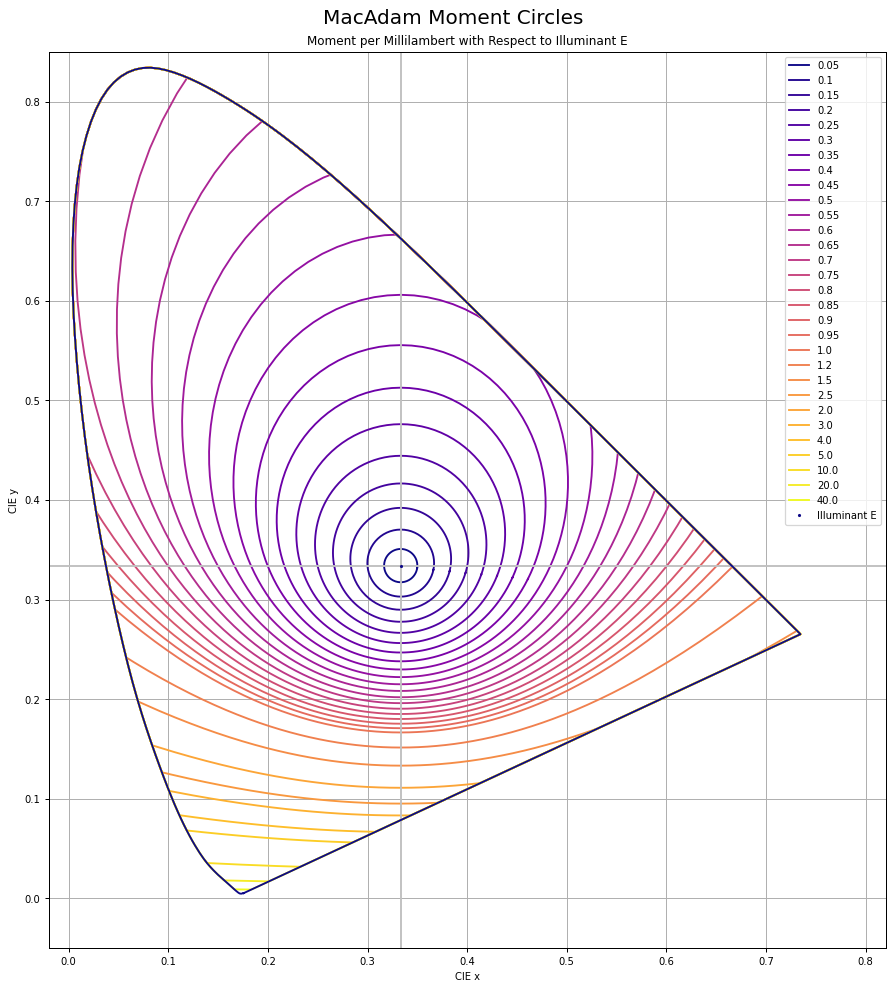
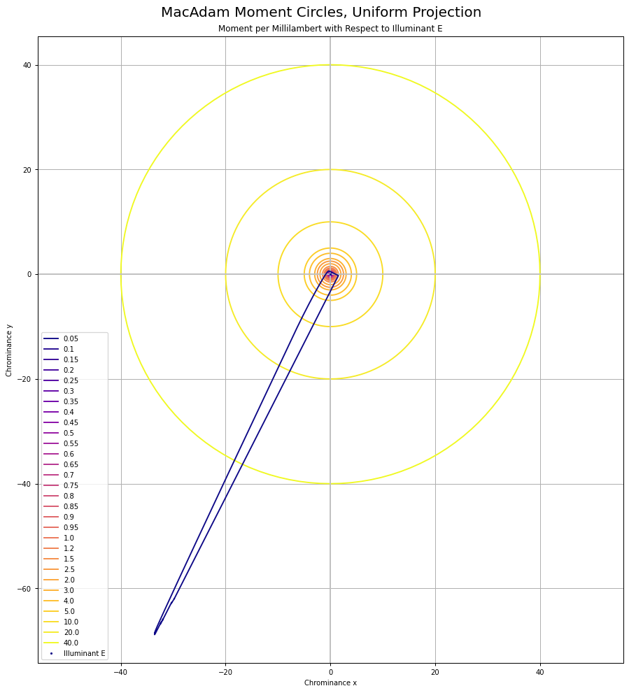
Chrominance follows the MacAdam work. I’ve recreated the original MacAdam diagram using a “uniform projection” space, and sampling concentric circles, then reprojected back to CIE xy:

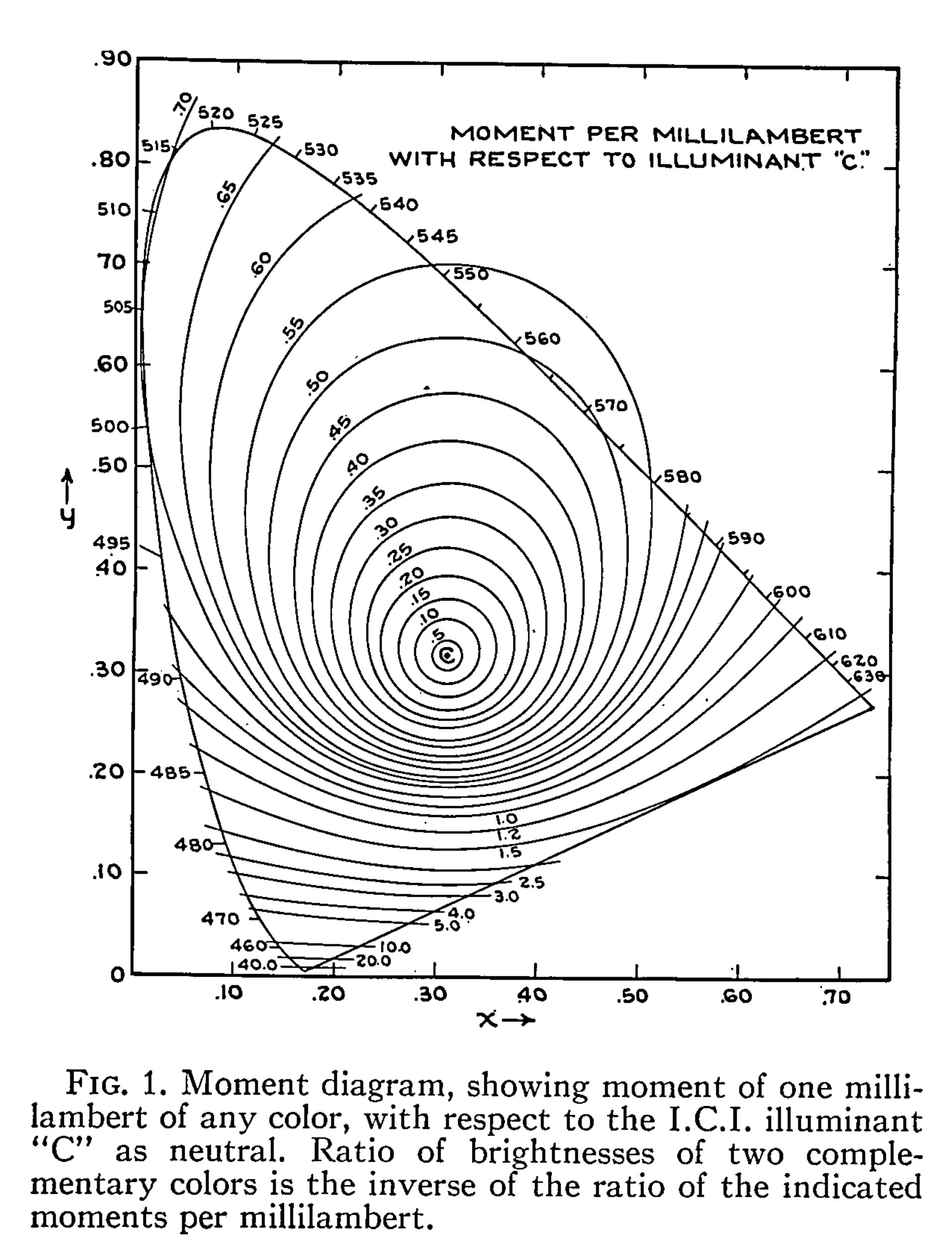
Here is the original diagram1 I was seeking to replicate:

We can calculate the ratios for any colinear CIE xy chromaticity through any arbitrary coordinate using a projection into a uniform vector space. It’s easiest to think of chrominance as the magnitude vector that forms from relative X to Z. Y remains isolated.

Oddly, I was unable to find any papers that cited the reprojection to a “uniform chrominance” projection. That projection looks like this when using the 1931 Observer system:

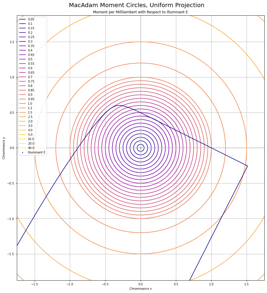
It can be useful to think of chrominance as the X to Z plane, with Y divided out to form an equi-energy projection. Here are the MacAdam “Moment” elliptical shapes, when projected into this equi-chrominance projection, cropped for clarity:

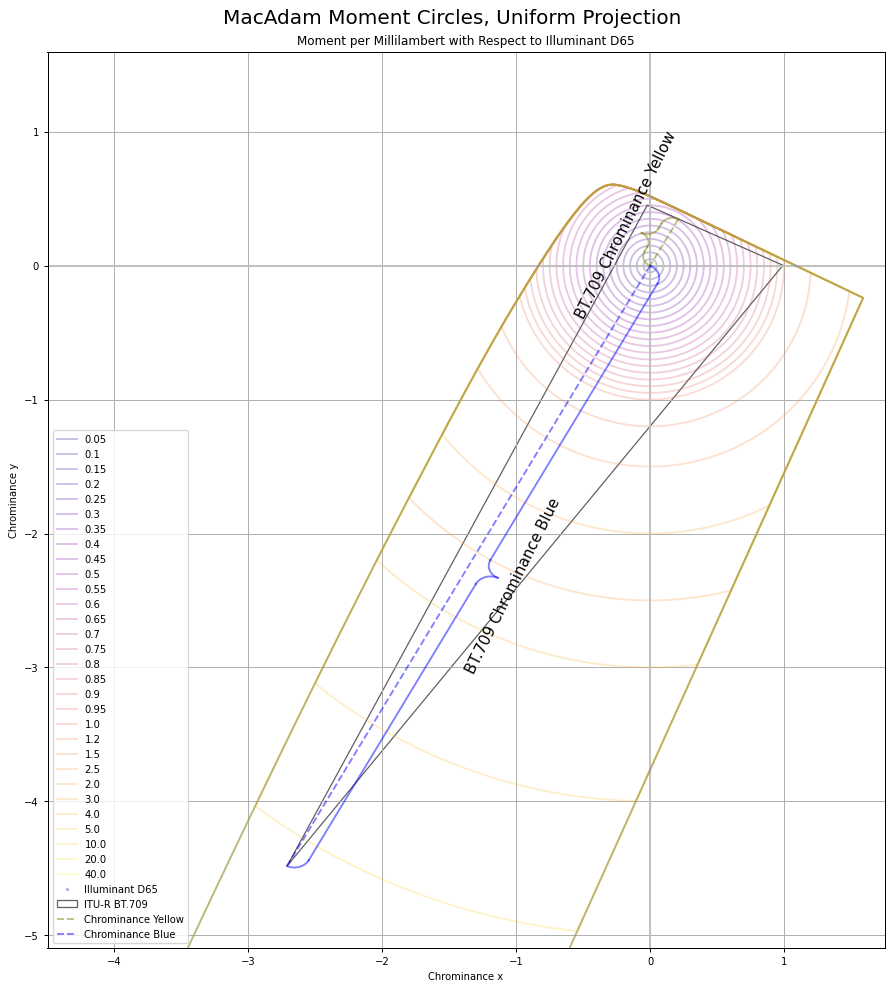
And here’s BT.709 projected into this chrominance plane:

The final “ratios” of underlying current stimulus are derived from the simple Euclidean distance ratios, which given they are ratios, plausibly is a direct line to the underlying differentials:

If we wander down this path of nonsense, total “neurophysiological” influence is the combined force of the resultant neurophysiological differentials, where “differentials” are not only the differences of the absorptive profiles, but the On-Off and Off-On assemblies:

  • The (P+D) signal can be broadly considered {Y}.
  • The combined vector magnitude of the (P-D) and (P+D)-T signal path is entwined in X to Z.

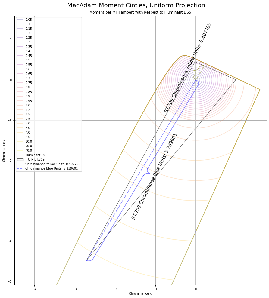
This means we should be able to calculate the ratios of gains of energy required to hit the target global frame achromatic using the ratios of either Y or the X to Z magnitudes. Using the projection above, the total Euclidean distance of the chrominance vectors is 5.239601 + 0.407705, for a total of 5.647306. If we divide each vector magnitude by the sum, we end up with the two cases for BT.709 “blue” and “yellow”:

  1. 0.407705 / 5.647306 which yields 0.07219460039.
  2. 5.239601 / 5.647306 which yields 0.9278053996.

If those resulting ratio values look awfully familiar to folks, they should. Those happen to be the luminance weights of BT.709 “blue” and “yellow” respectively.

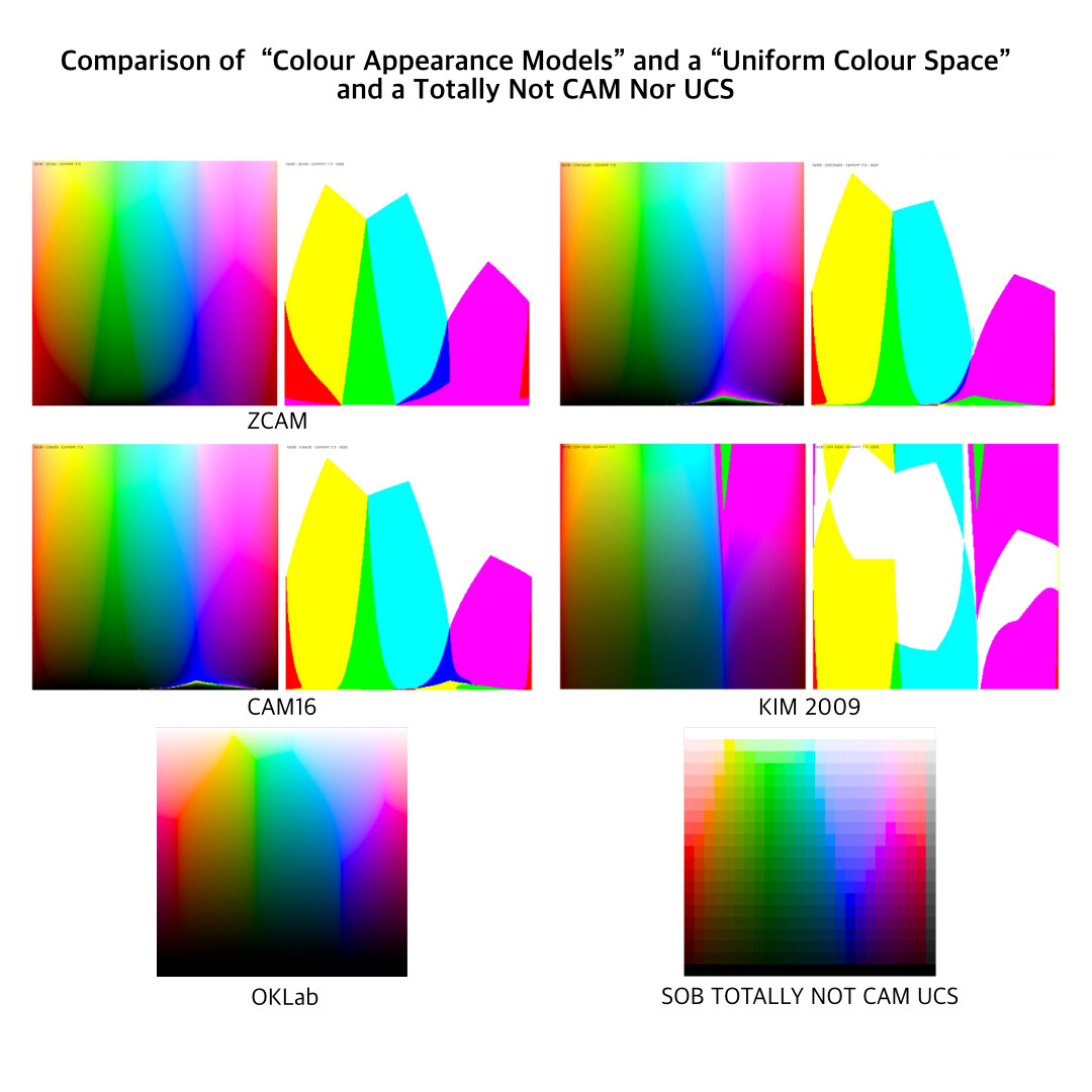
Incriminating Evidence against CAMs and UCSs

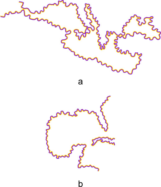
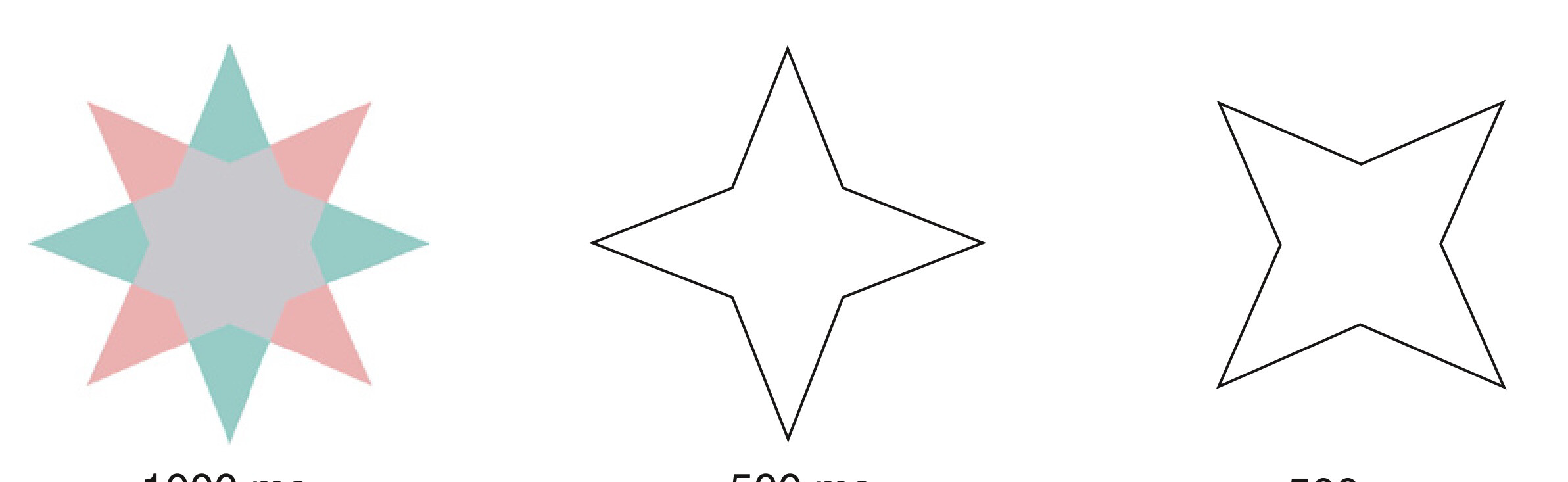
Moving along, if we consider literally all of the Colour Appearance Models and Uniform Colour Space attempts that have been made over the past half of a century, a peculiar trend line follows out of them. Let’s take a look by way of a post here on the forum, cropped, flipped, and collated against a Uniform Colour Model, and a Totally Not CAM / UCS Model from Yours Truly. The “model” I generated was simply a pure luminance mapping, with attenuation of purity to hit the target luminance, such as when a given luminance was unachievable at the mapping peg position. Note how all of the “clefts” in the CAMs match the exact clefts in the UCS, which in turn match the exact clefts in the luminance mapper:

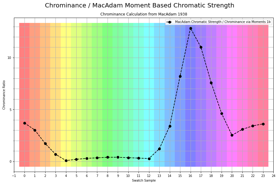
If we were to plot the chrominance ratios for a similar sweep of tristimulus using BT.709, it looks like this:

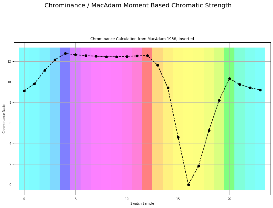
Here is the exact same measurement, inverted as over complementary values that accumulate to the achromatic Grassmann middle:

I believe it was Luke who, in the most recent meeting, stated:

The relationship between linear light and J is different than the relationship between linear light and M.

If we correct for that pattern, by way of gaining the underlying magnitudes of the tristimulus, I’ll leave it up to the reader to speculate with a wild guess as to what model we end up with if we were to indeed yield constant relationships between the chrominance ratio and the luminance ratio. Here is a passage of an example of the stated problem from the MacAdam original work:

Figure 1 can be used to advantage in any problem in which a neutral additive mixture is to be established. If, for instance, it is necessary to secure a white image on the screen in connection with an additive method of projection of colored photographs, suitable relative brightnesses of the three projection primaries can be readily determined.

Chrominance: The Shortcut

Given we are already often in balanced systems, working through the values from the Standard Observer has a direct shortcut. Chrominance is to Luminance as:

  1. Luminance = (R_w * R) + (G_w * G) + (B_w * B)
  2. Chrominance = max(RGB) - Luminance(RGB)

If that happens to look all too convenient, it is because RGB is already engineered to be a balanced system, and the underlying “force” gains are baked into the model. To recover the magnitude we just have to “extract” it.

Note the definition of chrominance here is following the one outlined by Boynton2, and is congruent with the other definitions such as those of Chromatic Strength, Complementation Valence, from folks such as Evans and Swenholt, Hurvich and Jameson, and Sinden:

We are now in a position to define a new term: chrominance. Whereas luminance refers to a weighted measure of stimulus energy, which takes into account the spectral sensitivity of the eye to brightness, chrominance refers to a weighted measure of stimulus energy, which takes into account the spectral sensitivity of the eye to color.

The simple description is that vector magnitude between X to Z.

1 MacAdam, David L. “Photometric Relationships Between Complementary Colors*.” Journal of the Optical Society of America 28, no. 4 (April 1, 1938): 103. Photometric Relationships Between Complementary Colors*.

2Boynton, Robert M. “Theory of Color Vision.” Journal of the Optical Society of America 50, no. 10 (October 1, 1960): 929. Theory of Color Vision.

5 Likes