Output Transform Tone Scale

More Tonescale Sigmoid Ramblings

The last couple weeks I’ve been doing some more explorations on this topic. I’ll summarize some of the more interesting points and thought-processes here for those rare persons who might still be following this thread.

A Tale of Two Contrasts

At the end of this meeting, I did a quick demo of the different behavior of contrast / exponent adjustments between these two functions

Daniele’s “Michaelis-Menten Spring Function”
f\left(x\right)=s_{1}\left(\frac{x}{s_{0}+x}\right)^{p}
where s_{0}=e_{0}s_{1}^{\frac{1}{p}} and e_{0} is the scene-linear exposure control.

the “Naka-Rushton Function” I posted before
f\left(x\right)=\frac{s_{1}x^{p}}{s_{0}+x^{p}}

The difference between the two functions is essentially where the exponent is applied.

  • In Daniele’s function, contrast is adjusted as a power function in display-linear.
  • In the Naka-Rushton function, contrast is adjusted as a power function in scene-linear.

Based on all the dumb experiments I’ve done with the above two tonescale functions, it seems necessary to have more contrast in SDR than HDR. This implies the slope through middle grey changes subtly between an SDR rendering and an HDR rendering. Logically this makes sense: Since we have more dynamic range available in HDR, we would want to have less highlight compression and less stretching of mid-range values through boosted contrast. The question I’ve been exploring is how do you create a tonescale that continuously changes between SDR at 100 nits peak luminance and HDR at > 1000 nits peak luminance?

What the heck is a spring function?!

I think Daniele used this term in one of the previous meetings (or maybe I imagined it, just like I think I imagined @SeanCooper using the term “water vs balloon” to describe display gamut rendering methods). Or maybe I just have a psychological vulnerability for inventing stupid names for things.

Anyway spring just refers to a sigmoid function which can be scaled in Y without the slope through the origin changing. A simple example being f(x)=s_{1}\frac{x}{s_{1}+x}. With this function you can multiply up s_1 and the slope through the origin stays constant, while the rest of the sigmoid is scaled up vertically. This way of thinking about HDR display rendering tonescales is much more elegant and simple than the messy way I was thinking about this before.

The basic approach is to

  • Set contrast with the power function
  • Set “exposure” or middle grey point using the scene-linear exposure control
  • Set peak white luminance using the y scale s_1.

Naka-Rushton Spring?

It’s easy to set up a “Naka-Rushton” equation in “spring” mode: f\left(x\right)=\frac{s_{1}x^{p}}{s_{0}+x^{p}}
where s_{0}\ =\frac{s_{1}}{e_{0}} and e_0 is our scene-linear scale.

As a simple example, here is a variation on the tonescale model based on the “Naka-Rushton Tonescale Function” I posted previously. It has a constant contrast of p=1.2, constant flare compansation of f_l=0.02, and maps middle grey to 10 nits at 100 nits peak luminance.

In this model, the output y-scale is normalized so that at 100 nits peak luminance, output display-linear = 1.0, then as peak luminance increases the output peak y value increases up to 40 at 4000 nits. To normalize into a pq range where 1.0 = 10,000 nits and 0.01 = 100 nits, you would divide by 100. This makes it simple to turn on pq normalization for HDR or turn it off for SDR.

As I hinted at before, I think we would want to reduce the contrast with increasing peak luminance. With a contrast of 1.2 at 4000 nits I think the highlights are pushed too bright. Or maybe this is a problem with the tonescale function, and the reason Daniele was asking “how does it work in HDR?”

Pivoted Contrast?

After the above description of the “Naka-Rushton” function, you might be thinking

Gee if that function is just applying a power function to scene-linear input data, why not turn it into a pivoted contrast function instead, so that middle-grey isn’t shifted around when adjusting contrast?!

It actually seems like a valid approach using something like a 3-stage tonescale rendering:

  1. Scene-referred pivoted contrast adjustment (possibly with linear extension above pivot)
  2. Scene-linear to display-linear rendering using pure Michaelis-Menten function
  3. Flare compensation

Many Valid Approaches

Given the large quantity of garbage in my previous posts in this thread I thought it might be useful to assemble a list of tonescale functions into a single place.

In this notebook there are 3 categories of tonescale functions

  • Michaelis-Menten : \frac{s_{1}x}{s_{0}+x}
    Just a pure Michaelis-Menten function, no exponent, no contrast.
  • Michaelis-Menten Display Post-Tonemap Contrast : s_{1}\left(\frac{x}{s_{0}+x}\right)^{p}
    The variation Daniele posted, with exponent applied in the display-referred domain.
  • Michaelis-Menten Scene Pre-Tonemap Contrast : \frac{s_{1}x^{p}}{s_{0}+x^{p}}
    The variation I posted above with the exponent applied in the scene-referred domain.

I have included “spring function” variations, and variations with intersection constraints where possible.

A Note on Names

Just a brief interlude to justify my decisions against @Troy_James_Sobotka 's pedantic trolling in the previous meeting.

In the original Naka-Rushton 1966 paper, the function they use is a classic Michaelis-Menten function y=s_{1}\frac{x}{x+s_{0}}. I agree that strictly speaking using this name to refer to my above function is disingenuous.

I used this name because in this other paper the “Naka-Rushton equation” is referenced as f\left(x\right)=s_{1}\frac{x^{p}}{s_{0}^{p}+x^{p}}.

Also technically speaking the function Daniele posted is a Michaelis-Menten function with an added contrast. Michaelis-Menten refers strictly to the hyperbolic function \frac{s_{1}x}{s_{0}+x}

So yeah, maybe moving forward we call these functions by what they are: The Michaelis-Menten function with contrast added in display-referred domain or scene-referred domain.

4 Likes

Michaelis-Menten Scene-Contrast

Here is another idea: If we apply contrast in the scene-linear domain using a pivoted power function with linear extension, and use a “pure” michaelis-menten equation with no exponent, you can almost get reasonably consistent results from 108-4000 nits peak brightness with a constant contrast setting.


m01 above ignores SDR and treats DCI 108 nit / 7.5 nit HDR as a valid datapoint in the spectrum of peak brightnesses.


m02 is a continuous range in middle grey from 10 nits at 100 nit peak, through 16 nits at 4000 nit peak.

5 Likes

Please keep those coming, I’m certainly lacking of time but this is great stuff that I have been enjoying between boring builds :slight_smile:

Is there a function you prefer in your latest batches?

Cheers,

Thomas

I will second Thomas’ comments, please do keep them coming.

Something I have been wondering about, is if only using peak output is appropriate for setting the parameters. I think we need to include the surround/adopting field luminance as one of the key parameters to allow us to understand how to bridge between dim and dark surrounds and to try rationalise the mid-grey luminance between the different outputs.

In a dark surround we assume the average picture luminance is scaled based upon the image luminance so we could make an assumption of ‘10%’ of peak for SDR when switching to Rec 1886 Output we switch our anchoring to be based on the reference surround value which by magic is also 10% of peak luminance. But when migrating to HDR this might break, so obviously we need to be a little more involved for choosing the mapping function, but this is just an off the cuff thought for consideration.

Kevin

1 Like

Yes please do keep those points coming. It is an interesting discussion to be had.

I’ll add my own grain of salt with regards to mapping SDR to HDR and I found that getting the black levels in the same place is important for a consistent experience given of course that both are viewed in the same viewing conditions.

1 Like

I put together a Tonescale Model Selects colab, with the most successful models in my trash pile of experiments.

I would say they all have different pros and cons.

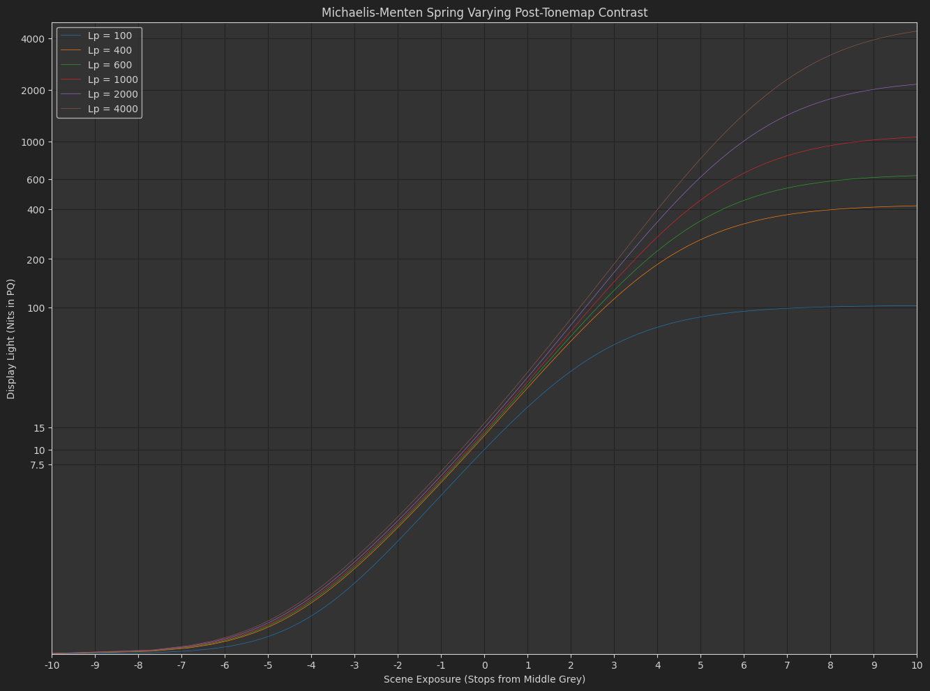
I like the simplicity and look of the pre-tonemap contrast with linear extension + michaelis-menten function. The Michaelis-Menten Spring Dual-Contrast model in the above colab is the one I will use moving forward I believe.

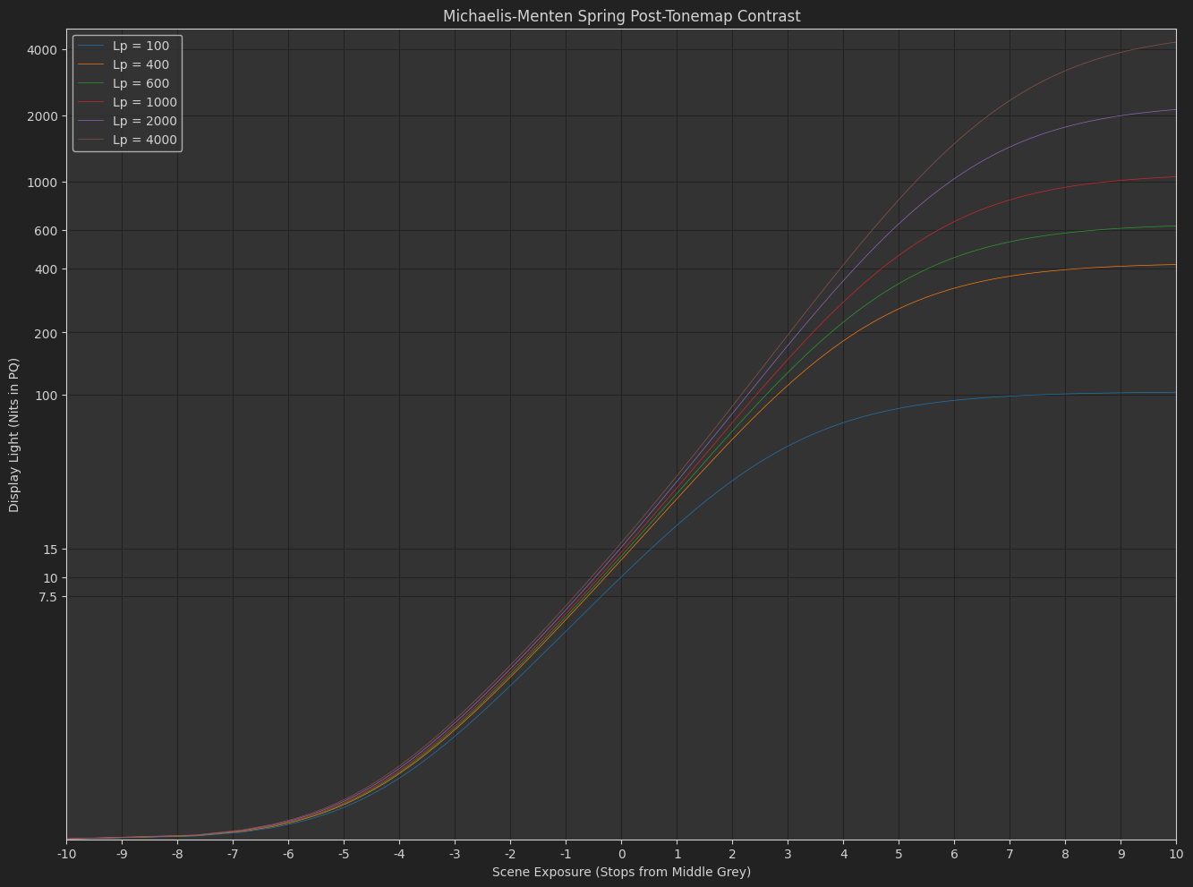
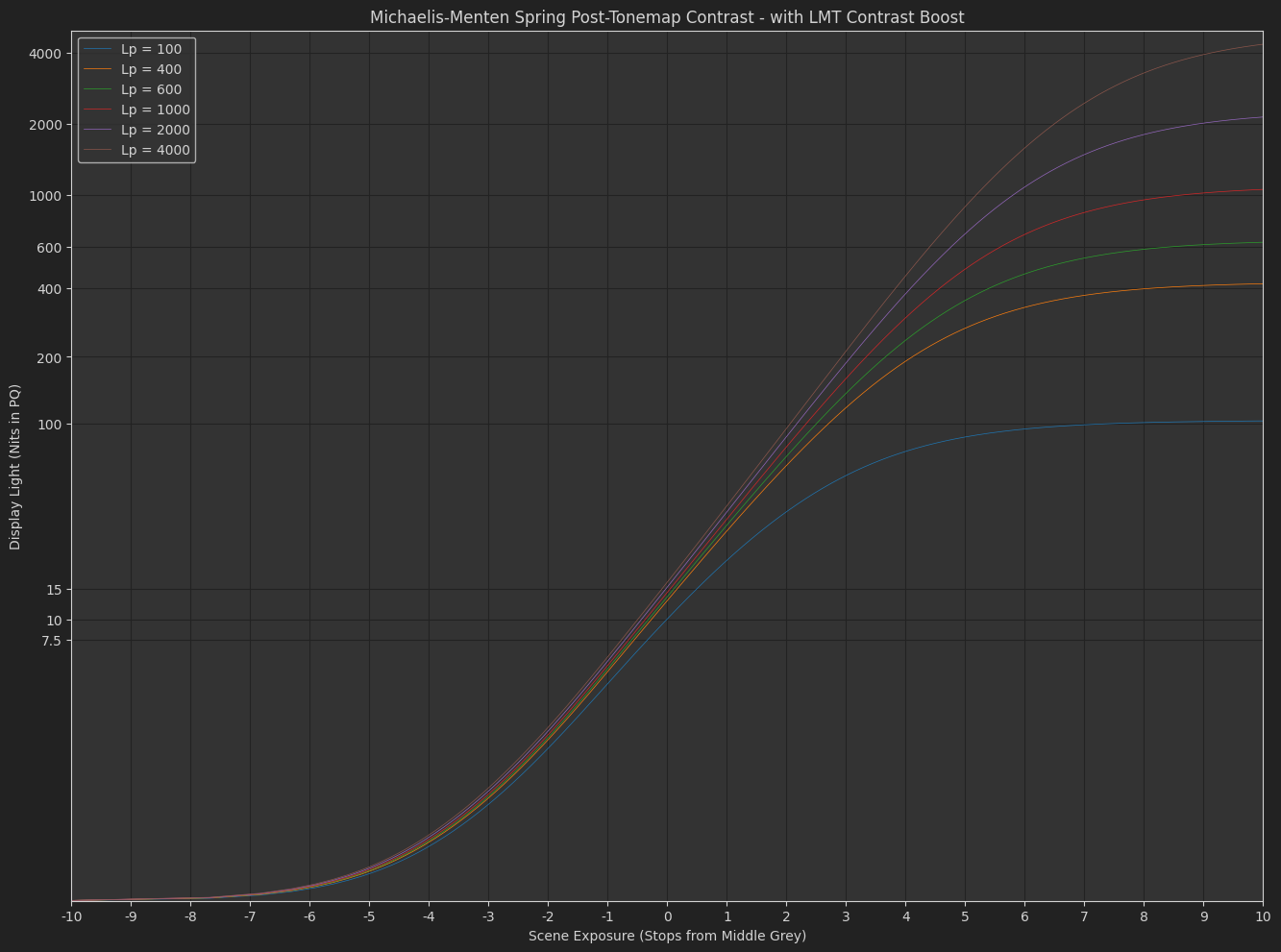
The post-tonemap contrast Michaelis-Menten Spring function is very neutral and performs very nicely in HDR, but the shadow contrast is too low in SDR. This is what I was previously fighting by modeling an exponent that started higher and decreased as peak luminance increased. I never liked this. Included in the Michaelis-Menten Spring model is an idea for a “default tonecurve lmt” which adds a bit of contrast to compensate and seems to work okay through the transition to HDR.

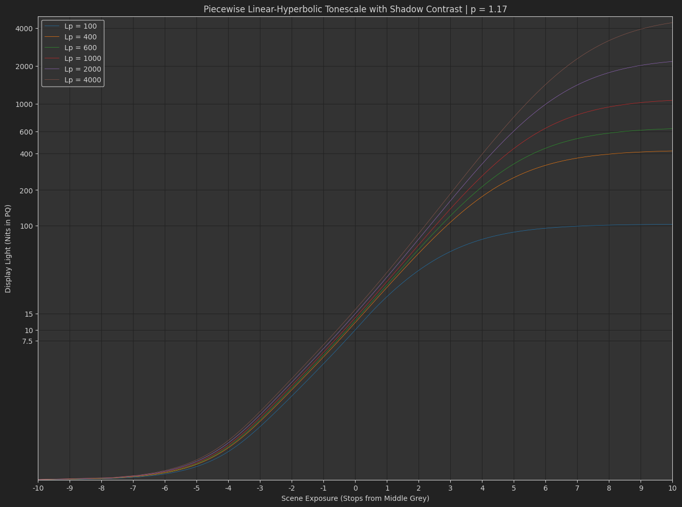
And I figured I would throw in a refinement of an earlier experiment with the Piecewise Hyperbolic Tonescale Model. In this one I do like that values below middle grey can be kept strictly linear if desired. It is more controllable. I also like the stronger highlight appearance, and the ease with which you can transition from SDR to HDR with a consistent contrast.

All models include a parameter for surround compensation using an unconstrained post-tonemap power function.

Tonescale_Selects_v01.nk (33.8 KB)
Here’s a nuke script with all the models as well.


I’ve also pushed OpenDRT v0.1.2 that uses the “dual contrast” tonescale model above.

7 Likes

While doing the OkishDRT I wanted to use the same tonescale as the ACES2 candidates use, the Michaelis-Menten Spring Dual-Contrast and needed its derivative to drive the path-to-white. It turns out there is a sudden transition in 0.18 where the tonescale changes from the linear extension to the michaelis-menten function, as seen in the following desmos plot: ACES2 MM-SDC tonecurve. Not sure if this is a problem for the tonescale but for using the derivative to do things it probably would be better if it was smooth.

I made a modified version of your Desmos plot, where C_1 is automatically calculated to make the curve continuous as you vary C_0, instead of being a slider.

You need to drop C_0 to 1.0 instead of 1.2 to make the first derivative smooth. That is probably not enough contrast for our purposes. But it is interesting to see where the kink comes from.

1 Like

My original suggestion was smooth in both derivatives.

2 Likes

I think that in fact when C_0 is set to 1.0, it becomes the same as your original function, does it not @daniele?

Edit: S_0 and S_1 also need to be set to 1.0, and l set to 0.05 to match the original Desmos plot you posted

Reposting this from earlier. Daniele’s tonescale in log plot to better see what the parameters do: Daniele Compression Curve

Here is my quick investigation code to fit a cubic polynomial, where by simple weighting it more closely matches at the join Google Colab.

And an updated graph ACES2 MM-SDC tonecurve

Here is a version of the tone scale formula which compensates for the reduction in exposure introduced by the (Display) Flare compensation.

As the first equation does not change the slope at zero (besides the gamma value) one could change the order without significant difference, but I find this cleaner.

t_1 as most of the parameters is there to give us leverage on many different issues at once.
Some are:

  • it compensates the display flare without moving 0.0; this is important in a relative black system
  • it compensates for the shadow wash-out, which is introduced by the first part of the equation
  • most importantly, it compensates for the kink you get from the toe of the log grading space toe, this is important for the “gradeability” of the system.

with t_1 = 0.0 we get a ACEScct to Rec.1886 mapping like this:


This makes grading in the working space very unenjoyable.

with t_1 = 0.01 we get a ACEScct to Rec.1886 mapping like this:


A bit better but still not good

with t_1 = 0.05 we get a ACEScct to Rec.1886 mapping like this:


Even better.

So the right value of t_1 is influenced by many factors, but mainly by the toe function of the default grading space and the EOTF of the display.

5 Likes

Seems quite easy to get very good match to the MM-SDC tonescale. I used following parameters: g = 1.1, w = 0.84, t1 = 0.075

To get exposure to match I had to adjust the w value. I haven’t checked whether HDR matches…


2 Likes

I’ve got a version of the ZCAM DRT (v013) that integrates @daniele’s new curve, along with @priikone’s values.

It can be found here if anyone want to have a poke:

2 Likes

The MM-SDC tonescale hit 1.0 quite early. With this new one ACEScct 1.0 output is 0.998 and with ACEScct 1.46799 the output is 0.9999. The toe t1 value should probably be a bit higher. But it’s all very close…

0-1 ACEScct:


Here’s Daniele’s tonescale for different peak luminances compared to MM-SDC:


SDR is a good match but HDR is different.

Nothing stops you to change w for HDR as the comment in the desmos already hints at.

Yes, and Jed figured out all this with his tonescales. So here’s a variant that now adjusts the exposure and the peak luminance also for closer match to MM-SDC. The exposure should be a match.

It adds a new parameter w1 that can be pre-computed and was derived in same fashion as in MM-SDC using Linear Regression. This parameter determines how quickly the curve hits the peak luminance.


HDR might now have a tiny bit more contrast compared to SDR. Don’t know how visible it is. Contrast too could be a parameter that changes a bit.

where do your destination values in the linear regression desmos come from.
I think it is unwise to scatter the origins of your constants in separate place.
Also it is a bit strange to have an analytical model be driven by an approximation to unknown data points.

I would try to express what those values should do and model that instead directly

1 Like