RGB Saturation Gamut Mapping Approach and a Comp/VFX Perspective

I’m not seeing the graft point when I try this. Isn’t the point that the first derivative of the curve at the graft point is 1.0, so it should be continuous? But I’m hitting the limit of my maths here, so could be wrong!

Wolfram Alpha solve for derivative at graft with a threshold of 0.8 and a limit of 1.0

we should not forget that we are talking about compressing RGB ratios and not luminance or something similar.
Anyway we are on the right track of discussion thanks to @jedsmith contribution.
We could start:

  • doing more tests
  • discussing shaper function (this is what we are doing already)
  • discussing thresholds for different use-cases
  • evaluate the parameter space
  • look for some possible caveats we need to be aware of
1 Like

I don’t see how not producing smooth gradients in any space is not an issue, seems like it has the potential for posterisation errors and not having smooth derivatives here makes me highly uncomfortable. Note that besides having continuous derivatives the hyperbolic tangent distributes the samples very regularly.

@nick : Is WolframAlpha displaying both parts of the function? It is visible rather clearly in Desmos.

Here is similar code, expressed in Mathematica, using Reinhart and a single limit.
This is the method I was referring to in today’s call and it seems functionally equivalent to the above. s is RGB saturation. No hue shift happens. Thanks, Danielle, for inspiring me to simplify my code.
It looks like alpha blending with a fixed color Max[rgb].
It preserves Max RGB.
BTW. Note the simplification of the Reinhart curve.

ToningCurve[inValue_, inRange_, outRange_] := 1/(1/inValue + 1/outRange - 1/inRange);

MapColorsTowardsKnee[rgb_, Limit_, Knee_] := Module[{
sIn, sOut, alpha, mappedRGB},
If[Max[rgb] - Min[rgb] <= Knee * Max[rgb], Return[rgb];];
sIn = (Max[rgb] - Min[rgb])/Max[rgb];
sOut = Knee + ToningCurve[sIn - Knee, Limit - Knee, 1 - Knee];
alpha = sOut / sIn;
mappedRGB = rgb * alpha + Max[rgb] * (1 - alpha);
Return[mappedRGB];
];

1 Like

No. I was just solving for the derivative of the compression function at the join, which comes out as 1. The function before the join is y = x, which obviously has a derivative of 1.

But I realise looking at the Desmos plot that while the first derivative matches at the join, it changes direction abruptly there, so the second derivative would not be continuous. Is that what you are referring to?

Yeah I was referring to C2 continuity!

Do you require C2 continuity?
Can we trivially tweak Reinhart curve to get that?

Good question!

It has not been stipulated as being a requirement but a few things to keep in mind:

  • The goal of this VWG is to propose a model that fixes artefacts. If we can do so knowing that the mathematical foundations are sound and will not produce some, the better.
  • When we authored the RAE paper in 2017, trying to get smooth derivatives was a strong wish for future updates of the RRT which is exhibiting quite a bit of wobbliness. The SSTS is authored with that in mind and it does make sense to continue that trend to me because it is a) good practise and b) a safety line.

I don’t know if it can be trivially done but would certainly be worthwhile.

Now besides that, I subjectively think that the Reinhart curve is doing a too much aggressive work and I don’t really like because of that. I think (and this is not subjective) that we should strive at keeping the maximum saturation possible, something OOG for ACEScg or BT.2020 is a very narrowband emitter and thus we should keep its saturated quality as long as possible.

Because a picture is worth a thousand words…

The image on the right certainly does not preserve either the physical, i.e. narrowband emitters, or the creative intent of the glowing spheres, the compression is simply too aggressive. People working at Animal Logic, e.g. @alexfry or Illumination, e.g. @ChrisBrejon are clients for such saturated imagery.

1 Like

And another simple example, a lambertian sphere lit with pure blue, red and green lights.

There are no specular at all in the shader but still, the Reinhart curve manages to produce some!

Cheers,

Thomas

Great example.
What do you mean by aggressive in this case?
Reducing over too wide a range?

The curves can be tweaked.
I use the R curve with a settable linear segment for the protected zone. I expect to set the knee at 0.8.
Tone[s_, Knee_] := If[s <= Knee, s, Knee + ToningCurve[s - Knee, inLimit - Knee, outLimit - Knee]];
Mapping range 0 to 2 to 0 to 1:
R curves with knees

Note that this curve maps max input to max output.
Can you share the original image? It’s a good test case.

Looking at the curve in the code sample above:
cd_r = d_r > thr ? thr+(-1/((d_r-thr)/(lim.x-thr)+1)+1)*(lim.x-thr) : d_r;
I reduced the math to:
thr + 1/(1/(dr - thr) + 1/(limx - thr))
This R curve cannot reach the desired upper bound, as it maps infinity to limx.
This is a known limitation of the classic R curve.
Consider this tweak:
thr + 1/(1/(dr - thr) + (1/(limx - thr) - 1/(maxIn - thr)) )
This curve maps maxIn to limx.

This curve is also trivially invertible, just negate the sign for the constant part. Watch out for the singularity.

2 Likes

Hey @LarsB,

I’m assuming you found the functions. Here is a pack for the imagery:

Cheers,

Thomas

PS: Nuke script for the terrible blue sphere render :slight_smile:

set cut_paste_input [stack 0]
version 12.1 v1
Camera2 {
 inputs 0
 translate {0 1 2}
 focal 15
 name Camera2
 selected true
 xpos 1280
 ypos 1938
}
Light2 {
 inputs 0
 color {0 0 2}
 translate {0 3 4}
 cast_shadows true
 depthmap_slope_bias 0.01
 name Light3
 selected true
 xpos 1290
 ypos 1842
}
Light2 {
 inputs 0
 color {0 4 0}
 translate {-0.5 1 1}
 cast_shadows true
 depthmap_slope_bias 0.01
 name Light2
 selected true
 xpos 1510
 ypos 1794
}
Light2 {
 inputs 0
 color {4 0 0}
 translate {0.5 1 1}
 cast_shadows true
 depthmap_slope_bias 0.01
 name Light1
 selected true
 xpos 1510
 ypos 1914
}
Diffuse {
 inputs 0
 name Diffuse2
 selected true
 xpos 1390
 ypos 1695
}
Cube {
 translate {0 -50 0}
 scaling {100 100 100}
 name Cube2
 selected true
 xpos 1390
 ypos 1743
}
push $cut_paste_input
Diffuse {
 name Diffuse1
 selected true
 xpos 1280
 ypos 1695
}
Sphere {
 rows 256
 columns 256
 translate {0 1 0}
 name Sphere1
 selected true
 xpos 1280
 ypos 1743
}
Scene {
 inputs 5
 name Scene2
 selected true
 xpos 1400
 ypos 1842
}
push 0
ScanlineRender {
 inputs 3
 conservative_shader_sampling false
 motion_vectors_type distance
 name ScanlineRender3
 selected true
 xpos 1390
 ypos 1959
}
ColorMatrix {
 matrix {
     {1.451439316 -0.2365107469 -0.2149285693}
     {-0.0765537733 1.1762297 -0.0996759265}
     {0.0083161484 -0.0060324498 0.9977163014}
   }
 name ACES2065-1_to_ACEScg5
 selected true
 xpos 1390
 ypos 1983
}
EXPTool {
 mode Stops
 red 2
 green 2
 blue 2
 name Exposure3
 selected true
 xpos 1390
 ypos 2007
}

1 Like

These are solid points, and aiming for “maximal” saturation is a terrific goal to put on this. There is literally one gamut mapping solution that addresses each per volume I believe, which is inherently bound by the quantisation bit depth.

That is, the noise floor that I believe @KevinJW brought up, is a byproduct of extreme saturated primaries incrementing in limited steps and resolving to an out of gamut value.

  1. The compression curve at the floor must be negotiated against the minimum quantisation increment and never result to an out of gamut value.
  2. The compression curve at the ceiling must be negotiated against the minimum quantisation increment and never result to an out of gamut value.

I may be completely wrong here, however I believe that amounts to precisely one curve that satisfies the top and bottom of the volume?

makes all sense @Thomas_Mansencal!

Parameterization

Thank you for the help with the math @LarsB (Goodness knows I need it! :slight_smile:)

As you are suggesting, I think it makes a lot of sense to to parameterize the algorithm by where the curve intersects 1.0, not by what value the asymptotic limit of the curve is. Doing this would make it easier to optimize distribution of the out of gamut values between the threshold and the gamut boundary.

When mapping from a camera gamut to a smaller gamut like ACEScg, the maximum inverse rgb ratio distance is known and could be optimized for.

When compressing the gamut of an ACEScg image which was converted from Alexa Wide Gamut, based on the position of the primaries of each gamut, the maximum possible distance would be calculable. For this example, it would be about r=1.06, g=1.06, b=1.2


In a VFX pipeline I could definitely see this as a tool with a functional set of parameters that would be optimized for the specific circumstance. For example on an Alexa Wide Gamut show, a comp supervisor might optimize the threshold and limit settings for an Alexa Wide Gamut to ACEScg gamut conversion. For a RED show this might be different. And for a full cg animation feature this might be a totally different process. Ideally this tool should be flexible enough in it’s parameterization to handle all scenarios elegantly.

Shaper Function
I’ve done a bit of poking around with sigmoid functions. The arctan sigmoid function might be a good compromise between tanh and Reinhard. The second derivative is smooth and the slope is less agressive than tanh. (Meaning that it doesn’t get flat as fast, or… the limit is approached less quickly. Forgive my mathematical neophyte terminology here…). This less agressive curve would reduce issues with invertibility which tanh definitely has in my testing so far.

You can see arctan graphed here in blue compared against tanh and R: arctan vs tanh vs. reinhard | Desmos

Sidenote: Would it be possible to parameterize the limit such that we define the value where the arctan curve intersects 1.0? (This is beyond my math capabilities I think).

Noise Threshold
Regarding handling of the noise floor: Would it make sense to add a lower threshold or rolloff such that if achromatic is lower than a certain value, the quantity of gamut compression would be reduced? If gamut compression is being inverted in a VFX pipeline I could definitely foresee issues with grain in the blacks getting wonky after a gamut uncompression. Technically we shouldn’t really consider negative values resulting from sensor noise as “out of gamut” should we?

1 Like

Your current code seems to adjust each component independently:

  cd_r = d_r > thr ? thr+(-1/((d_r-thr)/(lim.x-thr)+1)+1)*(lim.x-thr) : d_r;
  cd_g = d_g > thr ? thr+(-1/((d_g-thr)/(lim.y-thr)+1)+1)*(lim.y-thr) : d_g;
  cd_b = d_b > thr ? thr+(-1/((d_b-thr)/(lim.z-thr)+1)+1)*(lim.z-thr) : d_b;

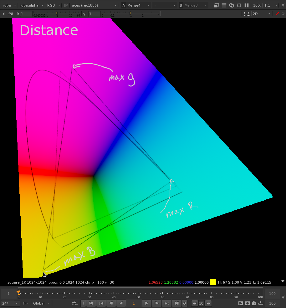
For example in rgb {1,2,3} 3 gets a stronger reduction than 1.
This causes significant hue shifts away from the RGB primaries. 10+ years ago I shared a chart on this with the ACES group but I can’t find it. Alex or Joseph might recall the chart or at least the red car that turned orange.
One way to avoid this is to have a single controller value.
In my code I now use straight alpha blending towards a gray color.

newrgb = alpha * rgb + (1 - alpha) * Max[rgb] * white;

You might want to give this a try.
This retains the RGB hue.
Do you consider alpha blending to be hue preserving?
(As the RGB space isn’t hue linear (there is no such space AFAIK) there is still a slight shift in perceptual hue)
There might be advantages to using alpha in addition to it preserving the hue.

  • Calculating one controlling value instead of three!
  • Maybe alpha and the gray background color can be smoothed or low res and applied in a separate step?
  • Maybe we can leverage some alpha blending optimizations??

That brings up an interesting Q;
What if we calculate the gamut map (alpha and background) at a lower res than the full image?
(and of course apply it to the full res)
Would this be OK or better for image integrity?
Or would it create edge artifacts?

The Limit
The max input can be calculated but maybe it’s overkill.
I have a 2020 to 709 reducer that maps 2020 edge to 709 edge.
This needs to be calculated for each pixel or at least each hue.
For performance reasons I want to get rid of it.
This is an optimized version that finds the 709 value that is equivalent to a 2020 value with same hue as rgb and one channel in 2020 being 0 - On the 2020 edge! Mtx709To2020 is a color space matrix from 709 to 2020.

maxIn = RGBtoSaturation[rgb - Min[Mtx709To2020.rgb ]];

Next, how do you use the limit?
Trivial for Reinhart. Not sure about the others.
After reading a BBC paper I tried using a log curve. Big problem, as in order to fit the curve, with C1 continuity, I had to calculate a scaling factor for each pixel and the math required solving product log, which was slow. I abandoned that curve model.

The conclusion is that for any chosen curve math you also have to have fast math for calculating its input to output range scale factors while maintaining C1 continuity. That’s why I’m pretty happy with Reinhart. But I’d like to see alternatives.

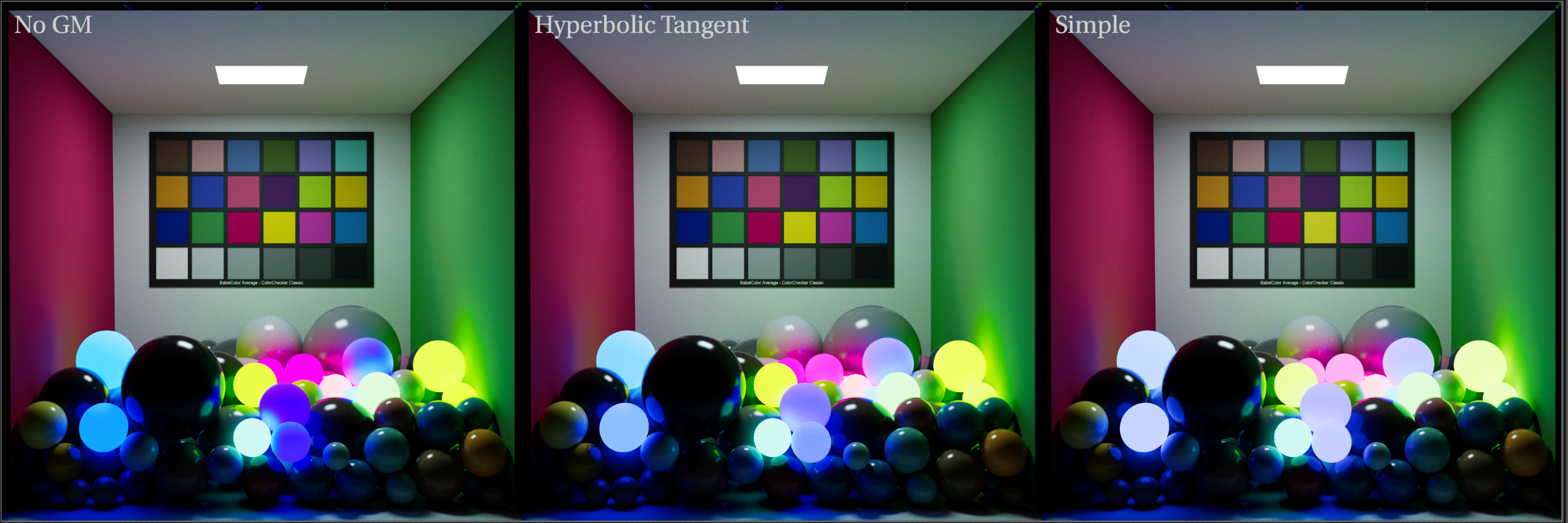
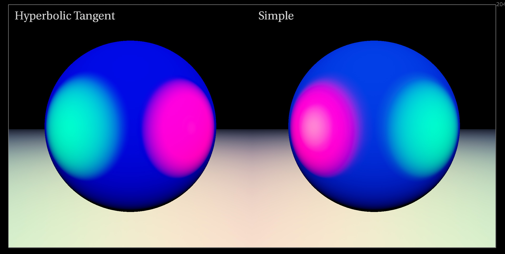
Regarding the curve shape.
Is there a significant visual difference if the various math curves are closely matching?
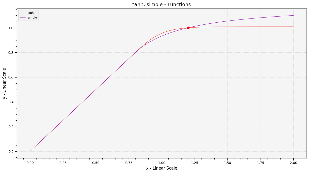
Maybe Reinhart’s simple math (1/1/x) is better for performance reasons? Can we do tanh in realtime on GPU?

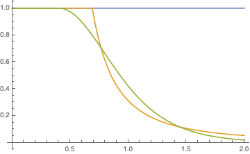
Here are two closely matching curves tanh (green) and reinhart (yellow).
They have different starting points (0.4 and 0.69) to make them match.
They have slightly different shapes. Does it actually make a visual difference?
image
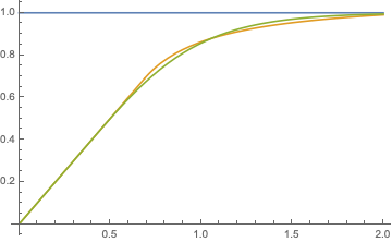
And here are the derivatives.
tanh has C2 continuity? Does it actually make a visual difference?
Is there any other aspect than visual appearance that we need to consider?
image

Sure does work, using it everyday. It is certainly much more expensive than the few ops from Reinhart but nothing that will scare a GPU.

My DCTL version of @jedsmith’s code (I hesitate to call it mine now, as Jed’s pull requests have pretty much rewritten it) includes the tanh option. It has no problem running in real time.

If not easily analytically derivable, it can be trivially solved, I added a notebook to do that here: gamut-mapping-ramblings/notebooks/gamut_mapping_compression_functions_01.ipynb at master · colour-science/gamut-mapping-ramblings · GitHub

And here is a copy on Google Colab (I will not maintain it though): Google Colab

Cheers,

Thomas