I have just updated my repo to include a Matchbox shader version for Flame (tested only on Flame 2021.)
tanh as toning curve has a major issue with invertability.
tanh maps Infinity a boundary value. Great.
But the inverse mapping arctanh maps boundary to infinity.
And it’s possible the inverse map will get such boundary values as input.
It seems we’d be better off with a curve that doesn’t go entirely flat.
ITU-R BT.2446 uses this curve, where K controls the compression above the threshold.
x<=1 ? x : 1 + K* ln((x - 1)/K + 1)
Disadvantages: Must solve ProductLog to determine K. Only C1 continuity
It is indeed a theoretical issue but not a practical one because you slightly clamp the values so that they never reach one or the limit you have defined. If you have such values anyway they are probably already so far off that you should have dealt with them upfront in the first place.
BT.2446 is certainly worth a look.
BT.2446 includes three methods ABC for mapping HLG HDR (2020, 1000 peak) to SDR (2020, 100 peak)
All methods are invertible.
Tone Mapping uses luminance.
They use different curves. Complex, not disclosed but looks like log & log.
B and C methods effectively use linear scaling in RGB. rgbOut= rgbin*Yout/Yin)
A does some chroma scaling.
RGB hue is preserved.
Using luminance seems weak.
All methods maps HDR mid blue (0,0,0.4) to SDR values > (0,0,1), such as (0,0,3). So not a sufficient gamut mapping.
B and C methods are quite simple, just using a toning curve. Here’s a code snippet for C:
CHDRLinearTo2020Linear[rgb_] := (
RGB = rgb;
Yin = LHDR * (rgb2Y.RGB);
If[Yin != 0, (
Yout = If[Yin < Yhdrip, k1 * Yin, k2 * Log[Yin/Yhdrip - k3] + k4];
RGB = RGB * ((LHDR*Yout)/(SDRReferenceNits * Yin));
)];
Return[RGB];
);
One constraint to consider is the max compression (or local contrast reduction)
When inverted this becomes max expansion (or local contrast increase).
Can we expand with a factor 16? This means that the expanded version will lose 4 bits in bit depth.
If 16 is OK, but 32 is not, this then sets the limit for the compression slope to be >= 1/16.
I just picked 16 as an example. Any idea what expansion factor we can use before we see banding, especially for noise-free content?
I’ve pushed a few changes to the gamut-compress git repo.
- Added DCTL versions of the code matching the latest restructuring I’ve done (thanks to @nick for the initial version!)
- The master branch still only has the reinhard compression curve. I feel like all of the other compression curves are a moving target and are experimental, thus I hesitate to call it “releasable”. Therefore it lives in the dev branch for now.
- The dev branch has all compression curves that we’ve come up with so far enabled (reinhard, exponent, arctan, tanh), and has the parameterization working properly to allow the user to specify the distance at which the curve intersects the gamut boundary. This needed a solver to calculate the intersection point, so it adds a bit of computational overhead for all compression curve types except Reinhard. For blinkscript this computation happens only when the user adjusts one of the max distance controls, not per pixel. For DCTL I’m not aware of a way to do pre-computation before entering the processing loop. Maybe @nick knows some secret way to do this? Anyway when testing I haven’t noticed any slowdown, so maybe the DCTL gpu compilation is smart enough to figure it out. Or maybe GPUs are just really fast.
I don’t believe DCTL has any way to run the equivalent of Blink’s init() function. Everything runs per pixel AFAIK. Unless there are some hidden optimisations.
Jed, I like the simplicity of the code.
BUT. this causes hue shifts in RGB space as you’re scaling the components with different values.
compress should be a scalar, calculated from the scalar ach.
This would remove the hue shift.
Here are the Munsell charts I showed in the meeting (Redone for AP0)
Munsell colors and AP0.pdf (189.2 KB)
I brought up the issue of clipping to gamut corners.
Hm, it’s probably not an issue for AP0 to AP1. Sorry for the distraction.
AP1 corners are on the spectrum locus so (as Matthias mentioned) there are no real colors outside those corners.
You see some unreal blues being clipped from AP0 to AP1 in the chart.
AP0 to AP1.pdf (46.8 KB)
This corner case is a real issue when mapping 2020 to 709, though.
Chart 2020 to 709.pdf (43.1 KB)
Here
ITP is defined in Rec. ITU-R BT.2124-0 Objective metric for the assessment of the potential visibility of colour differences in television.
ITP is a tweak of ICtCp
ITP = {1.0, 0.5, 1.0} * ICtCp
I think this 0.5 was for better error metric.
JAB is JzAzBz specified in Perceptually uniform color space for image signals including high dynamic range and wide gamut, MUHAMMAD SAFDAR et al, 2017
JzAzBz is a tweak of ICtCp.
I’ve updated my fork of @Thomas_Mansencal’s notebook so you can choose a Display P3 view transform (ACES or ‘naive’) for those who want to look at the result of the gamut compression on a wide gamut display, if they have one.
These are excellent plots Mr. Borg, so thank you for them.
I’m curious what is going on in your xy plot however. The curves appear to extend out to the spectral locus in the AP0 case, but I don’t recall the Munsell chipset being nearly that saturated.
Did you extend the plots using curve solved estimations?
The Munsell data set is from the Munsell Color Science Laboratory at RIT:
https://www.rit.edu/cos/colorscience/rc_munsell_renotation.php
In the 1940’s the color science community recognized that the most visually-uniform color space to date, the Munsell Color Order System, had inconsistencies that required examination and remedy.
all.dat: real and unreal
File download: all.dat
These are all the Munsell data, including the extrapolated colors. Note that extrapolated colors are in some cases unreal. That is, some lie outsize the Macadam limits.
This file should be used for those performing multidimensional interpolation to/from Munsell data. You will need the unreal colors in order to completely encompass the real colors, which is required to do the interpolation when near the Macadam limits.
I took a read through the BT.2446 paper. The log equation used for the upper portion of their tone-mapping algorithm looked useful.
Here’s a graph with all variables they have in their paper, comparing it to Reinhard and the natural exponential compression function, with variables modified to give similar y=1 intersection and threshold. And another graph, simplified, with d/dx, and inverse curve.
I’ve also implemented it in the GamutCompress blinkscript and DCTL. I need to do more extensive testing, but the initial results seem very nice. It feels a lot more natural than some of the other curves, and I haven’t yet noticed any issues from the lack of C2 continuity.
Now we have 5 different compression functions to test! ![]()
I’m also going to start using releases to track progress as @matthias.scharfenber suggested. Release v0.1 has only Reinhard compression and is working with a regular expression node and the blinkscript and DCTL.
Next step is to do a lot more testing regarding hue and results in different gamuts…
Nice! Will need to add it to the notebook, not sure if we want to try maintaining parity but it could be a good idea.
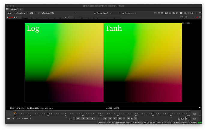
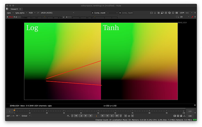
Visual inspection is certainly not enough because the eye is notoriously bad at detecting those type of low-frequency changes, where it starts being problematic is more with grading tools relying on qualifiers, here is some selective red suppression:
I can almost see a desaturated cone where the log variant starts kicking:
It gets worse by tweaking the distance limits. It might be a contrived example, but it is the type of things we should look for, especially because the operator will eventually be applied before grading.
set cut_paste_input [stack 0]
version 12.1 v1
push $cut_paste_input
Expression {
 expr0 "x / width - 0.25"
 expr1 "y / height - 0.25"
 name Expression14
 selected true
 xpos 3004
 ypos 2027
}
Group {
 name GamutCompress_blink9
 label "\[value method] : \[value direction]"
 selected true
 xpos 3004
 ypos 2051
 addUserKnob {20 GamutCompress}
 addUserKnob {4 method t "Choose the type of distance compression function you want to use" M {log reinhard exp atan tanh}}
 addUserKnob {22 reset -STARTLINE T "n = nuke.thisNode()\nknobs = \['threshold', 'cyan', 'magenta', 'yellow']\nfor k in knobs:\n    n\[k].setValue(0.2)"}
 addUserKnob {6 use_gpu l "use gpu" t "use gpu for blinkscript node" -STARTLINE}
 use_gpu true
 addUserKnob {7 threshold t "Percentage of the gamut to affect. A value of 0.2 will leave leave the core 80% of the colors within the gamut unaffected." R 0 0.2}
 threshold 0.3
 addUserKnob {26 distance_limit_label l " " t "Specifies the distance beyond the gamut boundary to map to the gamut boundary for each color component." T "<b>distance limit"}
 addUserKnob {7 cyan t "distance limit for the R component." R 0.001 1}
 cyan 0.2
 addUserKnob {7 magenta t "distance limit for the G component." R 0.001 1}
 magenta 0.2
 addUserKnob {7 yellow t "distance limit for the B component." R 0.001 1}
 yellow 0.2
 addUserKnob {26 ""}
 addUserKnob {4 direction M {forward inverse}}
 addUserKnob {20 info_tab l Info}
 addUserKnob {26 info_label l " " T "<style> a:link \{ color: #ccc \}</style>\n<font color=#ccc>\n<b>GamutCompress</b><br>\nmaps out of gamut colors back into gamut.<br><br>\n\n<b>Method</b><br>\nSpecify the tone compression curve to use when <br>\nmapping out of gamut colors into the boundary threshold.<br>\n<a href=https://www.desmos.com/calculator/hmzirlw7tj>log</a>\n<a href=https://www.desmos.com/calculator/lkhdtjbodx>reinhard</a>\n<a href=https://www.desmos.com/calculator/s2adnicmmr>exp</a>\n<a href=https://www.desmos.com/calculator/h96qmnozpo>atan</a>\n<a href=https://www.desmos.com/calculator/xiwliws24x>tanh</a>\n<br><br>\n\n<b>Threshold</b><br>\nPercentage of the gamut to affect. If threshold is 0.2, <br>\nthe inner 80% of the gamut will be unaffected and <br>\nout of gamut values will be compressed into <br>\nthe outer 20% of the gamut's color volume.<br><br>\n\n<b>Max Distance</b><br>\nPer color component control to specify what distance will be <br>\ncompressed to the gamut boundary. For example, <br>\na value of cyan=0.2 will map colors with a distance of red=1.2 from <br>\nthe achromatic axis to red=1.0, which is the gamut boundary.<br><br><br>\n\n<b>Direction</b><br>\nSpecifies whether to apply or inverse the gamut compression operation.\n<br><br>\n<a href=https://github.com/jedypod/gamut-compress>Additional Documentation</a><br><br>\n\nWritten by <a href=https://github.com/jedypod color=red>Jed Smith</a> with <a href=https://community.acescentral.com/t/rgb-saturation-gamut-mapping-approach-and-a-comp-vfx-perspective>help</a> from the <a href=https://community.acescentral.com/c/aces-development-acesnext/vwg-aces-gamut-mapping-working-group>ACES Gamut Mapping VWG</a>"}
}
 Input {
  inputs 0
  name Input
  xpos -40
  ypos -10
 }
 AddChannels {
  name AddChannels
  note_font Helvetica
  xpos -40
  ypos 26
 }
 BlinkScript {
  kernelSourceFile /cave/dev/github/gamut-compress/GamutCompress.cpp
  recompileCount 15
  ProgramGroup 1
  KernelDescription "2 \"GamutCompression\" iterate pixelWise 1dcee6a45b699c1349e8387e6472366b100957bee76685a075fd9740e0ab7c08 2 \"src\" Read Point \"dst\" Write Point 6 \"threshold\" Float 1 AAAAAA== \"cyan\" Float 1 AAAAAA== \"magenta\" Float 1 AAAAAA== \"yellow\" Float 1 AAAAAA== \"method\" Int 1 AAAAAA== \"invert\" Bool 1 AA== 6 \"threshold\" 1 1 \"cyan\" 1 1 \"magenta\" 1 1 \"yellow\" 1 1 \"method\" 1 1 \"invert\" 1 1 3 \"thr\" Float 1 1 AAAAAA== \"lim\" Float 3 1 AAAAAAAAAAAAAAAAAAAAAA== \"pi\" Float 1 1 AAAAAA=="
  kernelSource "kernel GamutCompression : ImageComputationKernel<ePixelWise> \{\n  Image<eRead, eAccessPoint, eEdgeClamped> src;\n  Image<eWrite> dst;\n\n  param:\n    float threshold;\n    float cyan;\n    float magenta;\n    float yellow;\n    int method; // compression method\n    bool invert;\n\n  local:\n  float thr;\n  float3 lim;\n  float pi;\n\n  void init() \{\n    pi = 3.14159265359;\n\n    // thr is the percentage of the core gamut to protect: the complement of threshold.\n    thr = (1 - threshold);\n        \n    // lim is the max distance from the gamut boundary that will be compressed\n    // 0 is a no-op, 1 will compress colors from a distance of 2.0 from achromatic to the gamut boundary\n    // if method is Reinhard, use the limit as-is\n    if (method == 0) \{\n      lim = float3(cyan+1, magenta+1, yellow+1);\n    \} else \{\n      // otherwise, we have to bruteforce the value of limit \n      // such that lim is the value of x where y=1 - also enforce sane ranges to avoid nans\n      // importantly, this runs once at the beginning of evaluation, NOT per-pixel!!!\n      lim = float3(\n        bisect(max(0.0001, cyan)+1), \n        bisect(max(0.0001, magenta)+1), \n        bisect(max(0.0001, yellow)+1));\n    \}\n  \}\n\n  // calculate hyperbolic tangent\n  float tanh( float in) \{\n    float f = exp(2.0f*in);\n    return (f-1.0f) / (f+1.0f);\n  \}\n\n  // calculate inverse hyperbolic tangent\n  float atanh( float in) \{\n    return log((1.0f+in)/(1.0f-in))/2.0f;\n  \}\n\n  // compression function which gives the y=1 x intersect at y=0\n  float f(float x, float k) \{\n    if (method == 0) \{\n      return k;\n    \} else if (method == 1) \{\n      // natural exponent compression method\n      return -log((-x+1)/(thr-x))*(-thr+x)+thr-k;\n    \} else if (method == 2) \{ \n      // natural logarithm compression method\n      return (exp((1-thr+thr*log(1-x)-x*thr*log(1-x))/(thr*(1-x))))*thr+x*thr-k;\n    \} else if (method == 3) \{\n      // arctangent compression method\n      return (2*tan( (pi*(1-thr))/(2*(x-thr)))*(x-thr))/pi+thr-k;\n    \} else if (method == 4) \{\n      // hyperbolic tangent compression method\n      return atanh((1-thr)/(x-thr))*(x-thr)+thr-k;\n    \}\n  \}\n\n  int sign(float x) \{\n    return x == 0 ? 0 : x > 0 ? 1 : 0;\n  \}\n\n  float bisect(float k) \{\n    // use a simple bisection algorithm to bruteforce the root of f\n    // returns an approximation of the value of limit \n    // such that the compression function intersects y=1 at desired value k\n    // this allows us to specify the max distance we will compress to the gamut boundary\n    \n    float a, b, c, y;\n    float tol = 0.0001; // accuracy of estimate\n    int nmax = 100; // max iterations\n\n\n    // set up reasonable initial guesses for each method given output ranges of each function\n    if (method == 2) \{\n      // natural logarithm needs a limit between -inf (linear), and 1 (clip)\n      a = -5;\n      b = 0.96;\n    \} else if (method == 4) \{\n      // tanh needs more precision\n      a = 1.000001;\n      b = 5;\n    \} else \{\n      a = 1.0001;\n      b = 5;\n    \}\n\n    if (sign(f(a, k)) == sign(f(b, k))) \{\n      // bad estimate. return something close to linear\n      if (method == 2) \{\n        return -100;\n      \} else \{\n        return 1.999999;\n      \}\n    \}\n    c = (a+b)/2;\n    y = f(c, k);\n    if (y == 0) \{\n      return c; // lucky guess\n    \}\n\n    int n = 1;\n    while ((fabs(y) > tol) && (n <= nmax)) \{\n      if (sign(y) == sign(f(a, k))) \{\n        a = c;\n      \} else \{\n        b = c;\n      \}\n      c = (a+b)/2;\n      y = f(c, k);\n      n += 1;\n    \}\n    return c;\n  \}\n\n\n  // calculate compressed distance\n  float compress(float dist, float lim) \{\n    float cdist;\n    if (dist < thr) \{\n      cdist = dist;\n    \} else \{\n      if (method == 0) \{\n        // simple Reinhard type compression suggested by Nick Shaw and Lars Borg\n        // https://community.acescentral.com/t/simplistic-gamut-mapping-approaches-in-nuke/2679/3\n        // https://community.acescentral.com/t/rgb-saturation-gamut-mapping-approach-and-a-comp-vfx-perspective/2715/52\n        // example plot: https://www.desmos.com/calculator/h2n8smtgkl\n        if (invert == 0) \{\n          cdist = thr + 1/(1/(dist - thr) + 1/(1 - thr) - 1/(lim - thr));\n        \} else \{\n          cdist = thr + 1/(1/(dist - thr) - 1/(1 - thr) + 1/(lim - thr));\n        \}\n      \} else if (method == 1) \{\n        // natural exponent compression method: plot https://www.desmos.com/calculator/jf99glamuc\n        if (invert == 0) \{\n          cdist = lim-(lim-thr)*exp(-(((dist-thr)*((1*lim)/(lim-thr))/lim)));\n        \} else \{\n          cdist = -log((dist-lim)/(thr-lim))*(-thr+lim)/1+thr;\n        \}\n      \} else if (method == 2) \{\n        // natural logarithm compression method: plot https://www.desmos.com/calculator/rv08vuzqjk\n        if (invert == 0) \{\n          cdist = thr*log(dist/thr-lim)-lim*thr*log(dist/thr-lim)+thr-thr*log(1-lim)+lim*thr*log(1-lim);\n        \} else \{\n          cdist = exp((dist-thr+thr*log(1-lim)-lim*thr*log(1-lim))/(thr*(1-lim)))*thr+lim*thr;\n        \}\n      \} else if (method == 3) \{\n        // arctangent compression method: plot https://www.desmos.com/calculator/olmjgev3sl\n        if (invert == 0) \{\n          cdist = thr + (lim - thr) * 2 / pi * atan(pi/2 * (dist - thr)/(lim - thr));\n        \} else \{\n          cdist = thr + (lim - thr) * 2 / pi * tan(pi/2 * (dist - thr)/(lim - thr));\n        \}\n      \} else if (method == 4) \{\n        // hyperbolic tangent compression method: plot https://www.desmos.com/calculator/sapcakq6t1\n        if (invert == 0) \{\n          cdist = thr + (lim - thr) * tanh( ( (dist- thr)/( lim-thr)));\n        \} else \{\n          cdist = thr + (lim - thr) * atanh( dist/( lim - thr) - thr/( lim - thr));\n        \}\n      \}\n    \}\n    return cdist;\n  \}\n\n\n  void process() \{\n    // source pixels\n    float3 rgb = float3(src().x, src().y, src().z);\n\n    // achromatic axis \n    float ach = max(rgb.x, max(rgb.y, rgb.z));\n\n    // distance from the achromatic axis for each color component aka inverse rgb ratios\n    // distance is normalized by achromatic, so that 1.0 is at gamut boundary, and avoiding 0 div\n    float3 dist = ach == 0 ? float3(0, 0, 0) : fabs(rgb-ach)/ach; \n\n    // compress distance with user controlled parameterized shaper function\n    float3 cdist = float3(\n      compress(dist.x, lim.x),\n      compress(dist.y, lim.y),\n      compress(dist.z, lim.z));\n\n    // recalculate rgb from compressed distance and achromatic\n    // effectively this scales each color component relative to achromatic axis by the compressed distance\n    float3 crgb = ach-cdist*ach;\n\n    // write to output\n    dst() = float4(crgb.x, crgb.y, crgb.z, src().w);\n  \}\n\};"
  useGPUIfAvailable {{parent.use_gpu}}
  rebuild ""
  GamutCompression_threshold {{parent.threshold}}
  GamutCompression_cyan {{parent.cyan}}
  GamutCompression_magenta {{parent.magenta}}
  GamutCompression_yellow {{parent.yellow}}
  GamutCompression_method {{parent.method}}
  GamutCompression_invert {{parent.direction}}
  rebuild_finalise ""
  name GamutCompress
  selected true
  xpos -40
  ypos 80
 }
 Output {
  name Output
  xpos -40
  ypos 134
 }
end_group
HueCorrect {
 hue {sat {}
   lum {}
   red {curve 0 0.25 1 1 1 1 0 s0}
   green {}
   blue {}
   r_sup {}
   g_sup {}
   b_sup {}
   sat_thrsh {}}
 name HueCorrect1
 selected true
 xpos 3004
 ypos 2083
}
The work that is being done here blows my mind, even though the math goes too much over my head 
Thanks so much for the matchbox version from @nick - I started playing around with it.
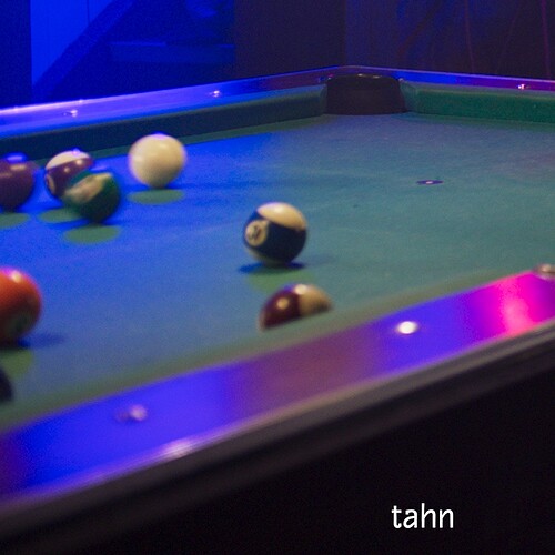
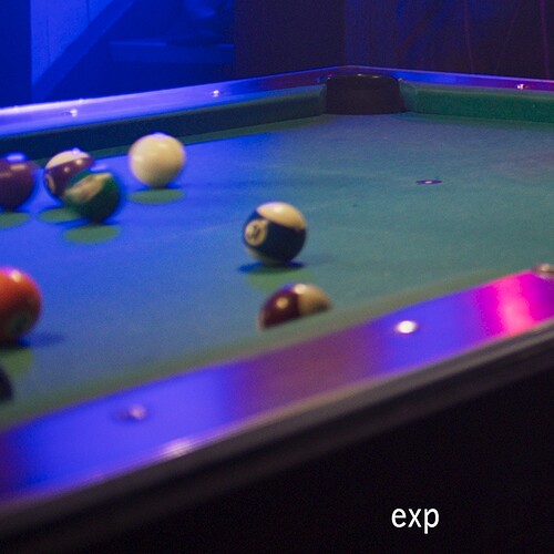
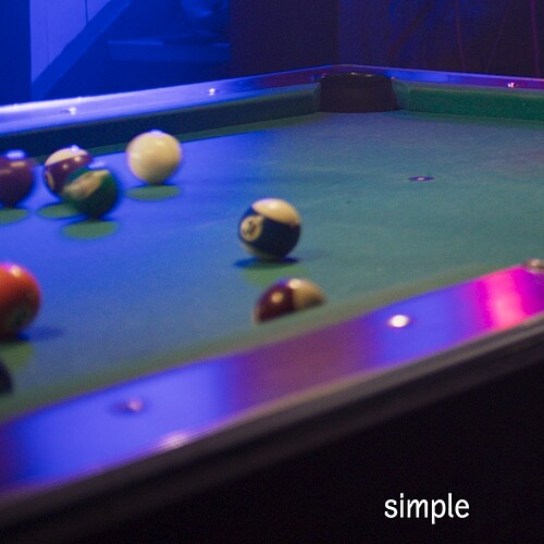
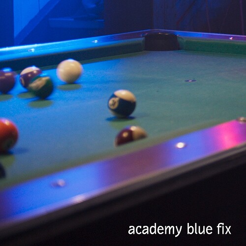
Right now I’m using the other frame from the take of the woman in the bar - I’ve also uploaded it to the dropbox repository.
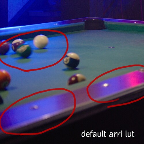
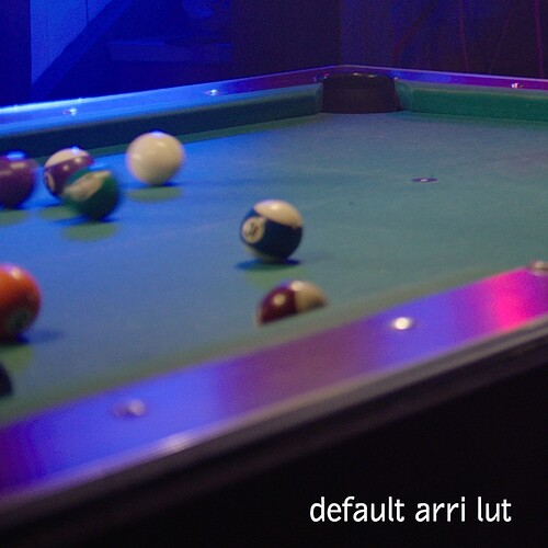
So this is how the image looks under default arri lut and this is what I use for kind of the best case scenario target, which I know is not really obtainable, but something to learn from.
I zoomed to this areas
these areas are interesting, because there are changes between colors which are quite sudden, but soft/gradient at the same time
so they are less “forgiving”
so this is the default arri lut
this is tahn
this is exp
this is simple
and this is the academy fix just for fun
all of the matchbox settings are default
I think all of them have their “problems”, but tahn is probably most pleasing, but still too dark and saturated
the shadows of the balls are especially “trippy” as the shadow should be darker, but it’s the other way around - I know it’s debatable, even the default arri doesn’t really do it like that and maybe even perceptually on the spot it would look darker…who knows…
and the other problems are the darker outlines - when the blue neon color blends into another one - green or brownish
tweaking the other parameters made the blue color brighter, which helps, but makes more visible outlines around the edges as a negative side effect
anyway, great to see the progress, I’ll take a look at the dctl version from @jedsmith next!
cheers!
Hey Martin!
Thanks so much for all the great imagery you’ve contributed for us to test with. It’s super important to have good test images, and the ones you’ve shared are super useful.
Interesting idea using the camera display lut to use as a sort of ground truth to compare against.
I’ve been playing around quite a bit with the different compression methods, and interestingly you can get pretty much the same results out of each compression method if you carefully adjust the threshold and max distance.
I think the max distance limit parameters are the critical thing to reduce undesired shifts in color and to keep as much saturation as possible.
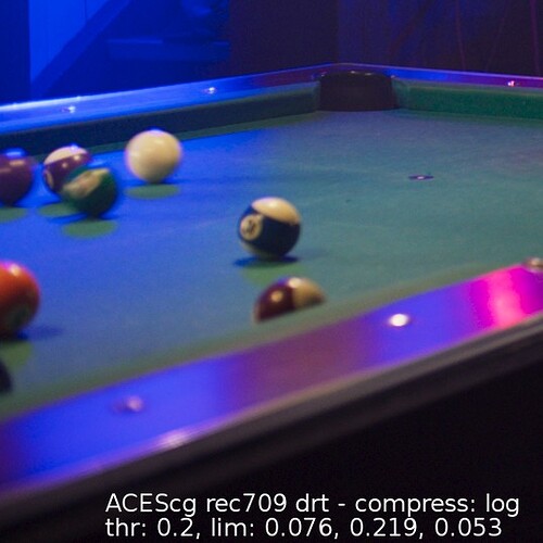
For example for compressing the gamut of an Alexa Wide Gamut source image in ACEScg, the max possible distance (assuming there are no out of gamut values in the source camera gamut image) is 1.07, 1.21, 1.05. If you plug these values into the cyan magenta yellow max distance limit controls you get a result that is pretty close to the Arri view lut.
Here’s a comparison. (I’m using the log compression method here but the same results should be present for the other options as well).
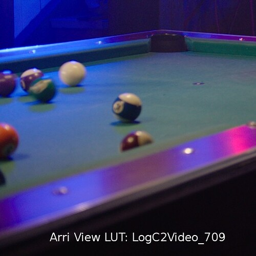
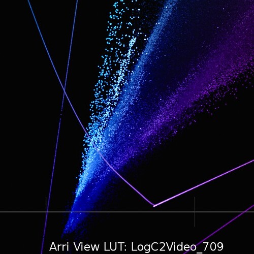
Arri LogC2Video_709 View Transform / Display Rendering Transform (DRT)
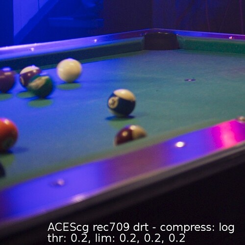
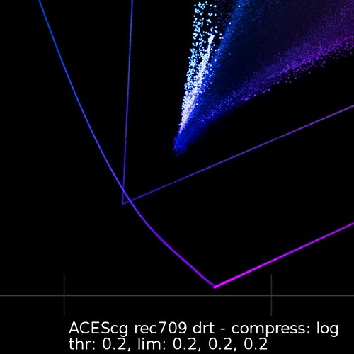
Arri Wide Gamut source image with IDT applied and gamut compress with default values in ACEScg. Note the purple shift in the light on the top of the pool table.
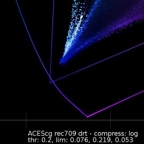
Same ACEScg image but with the max distance parameters of the gamut compress set to the max possible distance from an Alexa Wide Gamut → ACEScg mapping:
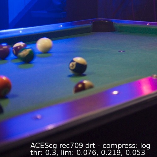
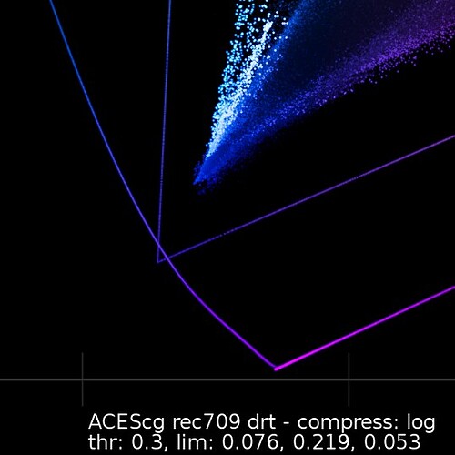
And for fun, here’s another with the threshold increased slightly so that we affect 30% of the outer gamut. The saturation is reduced a bit, because we are pulling the out of gamut values farther inside the gamut boundary.
And to help visualize what is going on, here is a CIE 1931 xy plot of the blue primary for each of these images:
With the default max distance limits, the Cyan corner of the triangle is over-compressed resulting in the purple shift.
With the max limit adjusted to the max possible distance for an Arri Wide Gamut → ACEScg mapping, the values are compressed more or less on a line straight through the blue primary of the source and destination gamuts. This reduces the purple shift.
From this:
- To get a “hue” accurate mapping is it necessary to set the max distance ratios according to the source gamut? How would you derive this or parameterize it? Presets for different common digital cinema cameras?
Also another update on the gamut-compress repo. I’ve added a “shadow rolloff” parameter. This is a control to smoothly reduce the effect of the gamut compression below a threshold achromatic value. The idea is to protect dark areas of the image which are primarily grain. This works by doing a Toe adjustment on the achromatic used for the division and multiplication portion of the distance calculation.
I think it works pretty well and actually reduces invertibility issues that were occurring in grain areas, where the distance values were going crazy due to the very small value of the denominator in the distance calculation.
I’ve also done a v0.2 release with all compression functions.
