Output Transform Tone Scale

daniele · September 12, 2022, 2:49pm

There seems to be a bit of confusion about the parameterization of the tone scale curve.
I made a pedagogical version with some helper lines, also I have changed the parameter space so it might become a bit clearer.
Also, it drove me mad that the Y-axis was not logarithmic while the x-axis was. So changed that as well. Now it should be log-log:

A short description:
N_r defines what nit level 1.0 in the linear light output axis means.
So if N_r is 100: The resulting output scale is:
1.0 = 100 nits
2.0 = 200 nits
10.0 = 1000 nits
100.0 = 10000 nits

If you want an output where the linear light output domain equals the nit scale set N_r = 1.0.
That would result in:
1.0 = 1 nits
2.0 = 2 nits
10.0 = 10 nits
100.0 = 100 nits
etc…
Ultimately, it does not matter if the EOTF encoding is scaled accordingly.
Be careful because the plumped Log Axis encoding in Desmos messes up all this.
N_r is not important for this discussion, so I moved it to the bottom

N
defines the display referred tone mapping target (relative to N_r), I added a list of a few values so we can see SDR and HDR at once.

r
defines which scene referred value should hit the display referred tone mapping target.
I added a little expression to make it be driven by n

I have replaced w with two parameters c for center and c_d for center display referred.
In addition, I added w_g to allow you to scale c_d when the Peak Luminance changes.

(Spoiler for the math nerds, the calculations of c_d are not exact. But the error is very small if r is very big, and the error plays into our direction ).

Thomas_Mansencal · September 14, 2022, 7:18am

Thanks this is great! Bonus points for the multiple curves at once, makes it really trivial to appreciate how some parameters are affecting the curve shape.

jeffrey.d.mathias · September 14, 2022, 3:57pm

Great… thanks for the log-log.

Question: Will the math of the ODT using these multiple Daniele curves be good enough to be used to automatically calculate what would be done with various trim passes (not totally, understood for aesthetic reasons.) But, if a grade is made at say either 1000nit, or 600nit, or 100nit, that other appropriate trims could be derived from that grade… and at what accuracy? And maybe considered another way, how much necessity will there be for additional trims? (sort of thinking work and time savings.)

sdyer · September 14, 2022, 6:24pm

@daniele thanks for the details and for the further parameterization

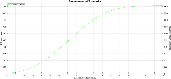
Here is Daniele’s function with the default values at 100 nits, and on a PQ y-axis (to better see the shadows).

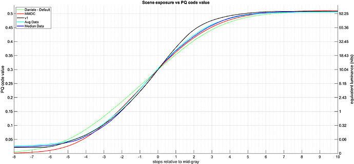
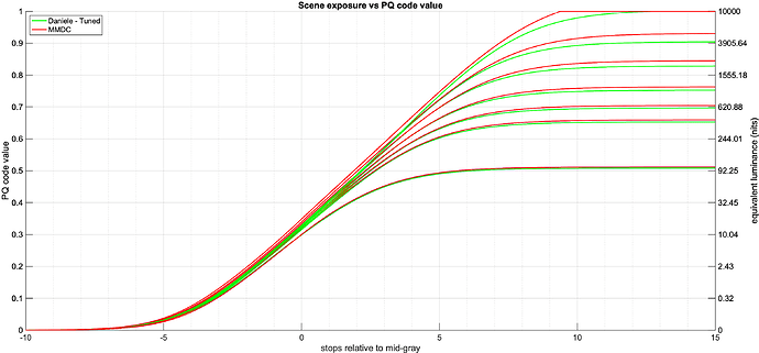
Now, let’s add @KevinJW’s “Avg Data” & “Median Data”, as well as “ACESv1 - 100nits”, and “MMDC” (aka the Jed curve used in 3 current test candidates).

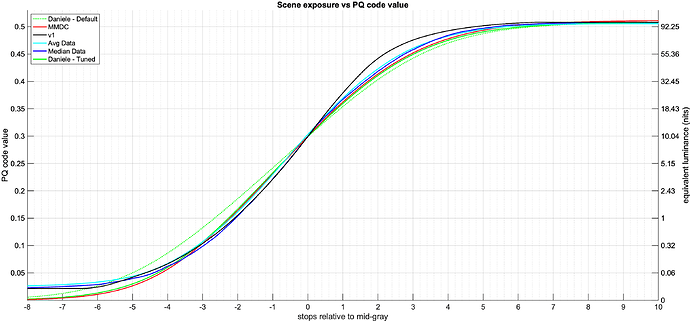
With the other curves also plotted, it is clear the default is quite a bit less contrasty than the other 4 curves, both in shadows and highlight rolloff. Therefore, I adjusted some of the values until I got something closer to what I think we’re aiming for:

This is using g = 1.2 to boost overall contrast and t_1 = 0.025 to pull the toe down a bit. I haven’t looked at any pictures with this yet, but from the plots at least, this should look pretty darn close to MMDC.

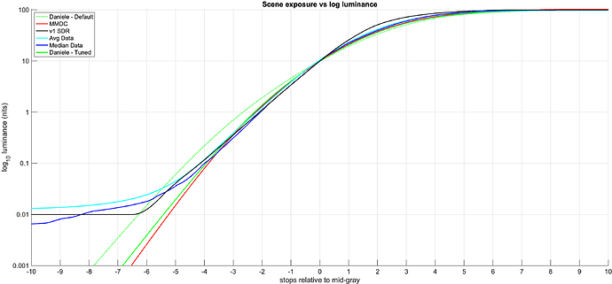
We can also compare them on log luminance y-axis.

HDR

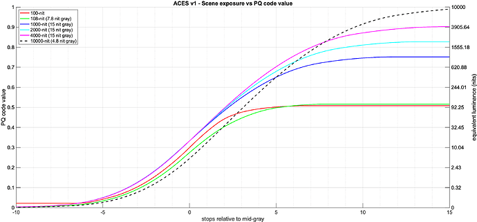
As we know, ACES v1 is a bit weird because it uses the two part tone scale for SDR and the single-stage tone scale (SSTS) for >100 nit peak luminance. Furthermore, the preset for 108 nits puts mid-gray at 7.2 nits, but the three presets for 1000, 2000, and 4000 nits all set mid-gray at 15 nits - creating a very unclear reasoning for where when and how mid-gray should increase in relation to the peak luminance target. For example, how should one use the SSTS to create an OT for 600 nits? What do I set mid-gray to? None of the curves have a clear relationship. Also the “RRT” (10000 nits) is defined through 4.8 nits, so this also is very confusing.

We know that we want the v2 tone scale to increase mid-gray slightly as peak luminance increases. Both MMDC and Daniele’s curve here have defined a relationship for that and behave well with increased peak luminance. (I adjusted w_g = 0.12 )

Questions

One of the items in the RAE was to be able to describe the origin of all “magic” numbers and parameters.
So can we justify where we put everything for these curves?

Was it ok to set the gamma higher in order to get it to closer match the other candidates?
What should be value of flare? Should it correlate to something real or ok to change value in order to bring toe of curve down closer to the other shapes?
What should be value of w_g?
Do the n_r values of [128, 256, 384] for [100, 1000, 10000] make sense?
Is 18% at 9.901 close enough to our aim of 10 nits? Or do we desire that it hit 10.0 on the dot?

Here are the values for 0.18 and 1.0 compared for various output peak luminance:

100 nits

ACES	Daniele -Tuned	MMDC	ACES v1
0.18	9.90	10.01	9.97
1.00	45.16	46.48	61.87

1000 nits

ACES	Daniele - Tuned	MMDC	ACES v1
0.18	13.36	14.08	15.00
1.00	101.26	103.39	107.44

2000 nits

ACES	Daniele - Tuned	MMDC	ACES v1
0.18	14.04	15.17	15.00
1.00	113.05	116.88	117.98

4000 nits

ACES	Daniele - Tuned	MMDC	ACES v1
0.18	14.33	16.32	15.00
1.00	119.93	129.18	126.85

10000 nits

ACES	Daniele - Tuned	MMDC	ACES v1
0.18	13.71	18.06	4.80
1.00	118.83	145.30	54.01

The big question for the group is “When can we “lock” the tonescale?” (and move on to focusing solely on the blues/reds and highlight rendering, etc.)

daniele · September 15, 2022, 3:54pm

You cannot precalculate everything I think, you end up chasing your own tail in the inverse precalculation.
So I checked where a round trip would produce a small error. If r_hit is inf the calculations are exact. If r_hit is smaller than inf the resulting c_d is a tiny bit smaller than predefined. (The error is also changed by changing g and t1). The error will scale inversely with N. In a way this is nice because the brighter we get the error reduces the increase of grey, so it is a nice “easy out”.

But there is a reflection point, which we need to avoid. According to your table, we reached the reflection point already. Check grey between your 4000 and 10000 nits. The 10000 nits grey value is smaller than the 4000 nits in your table. I get different values when I put in your tuned parameters: I tried your values and I get:

version	Input	Output
4000	0.18	0.150708806028
10000	0.18	0.150358120287

Still the 10000 nits is slightly lower than 4000 nits, this is because of your parameter tuning.

If you tune the parameter you need to keep an eye on that and tune w_g to avoid that the reflection point is below 10000 nits.

About r_hit,
I find it nice that you end on even numbers for 100, 1000 and 10000 nits, that’s all. I think it is convenient to remember.
To produce peak in SDR you need 128
To produce peak in 1000 nit HDR yo need 256

I think this is more practical for an artist that’s all.
You can use any number really, just remember the smaller the numbers the more errors the precalculation introduces.

About g
g of 1.2 is kind of a final value. It really depends if you want to produce the final contrast in the DRT. Colourists like to start on a slightly softer image and add contrast in the grading session

About t_1
Your value sounds a bit hard to me, remember we do not have a flare offset, so the function will compress shadows quite radically if t_1 is high.

p.s.:
(maybe someone can find a better precalculation method)

jeffrey.d.mathias · September 19, 2022, 4:38pm

I attempted a DCTL to play with Daniele’s function (below), but I seem to need some fixing in piecing together the output function.
+++

DEFINE_UI_PARAMS(n, Peak Luminance nits, DCTLUI_SLIDER_FLOAT, 1000.0, 100.0, 8000.0, 1.0)
DEFINE_UI_PARAMS(nr, Normalized White), DCTLUI_SLIDER_FLOAT, 100.0, 48.0, 200.0, 1.0)
DEFINE_UI_PARAMS(g, Suround-Contrast, DCTLUI_SLIDER_FLOAT, 1.043, 1.0, 1.3, 0.001)
DEFINE_UI_PARAMS(c, Scene Referred Grey, DCTLUI_SLIDER_FLOAT, 0.18, 0.09, 0.36, 0.01)
DEFINE_UI_PARAMS(cd, Display Referred Grey nits, DCTLUI_SLIDER_FLOAT, 10.0, .09, 20.0, 0.01)
DEFINE_UI_PARAMS(wg, Luminance delta Grey, DCTLUI_SLIDER_FLOAT, 0.0, 0.0, 1.0, 0.01)
DEFINE_UI_PARAMS(t, Shadow toe flare-glare comp, DCTLUI_SLIDER_FLOAT, 0.0, 0.0, 0.1, 0.01)

//n = [ 100, 250, 500, 1000, 2000, 4000, 8000 ] and nr = 100 NOTE: refine and simplify inputs

DEVICE float3 transform(int p_Width, int p_Height, int p_X, int p_Y, float p_R, float p_G, float p_B)
{

float3 rgb = make_float3(p_R, p_G, p_B);

float rhit = 128.0f + 256.0f * (_logf(n / nr) / _logf(10000.0f / 100.0f ));

float mo = n / nr; //NOTE: carefull with order of the following
float ma = 0.5f * (mo + _sqrtf(mo * (mo + 4.0f * t)));
float u = _powf((rhit / ma) / (rhit / ma) + 1.0f, g);
float m = ma / u;
float wi = _logf(n / 100.0f) / _logf(2.0f);
float ct = cd / nr * (1.f + wi * wg );
float gip = 0.5f * (ct + _sqrtf(ct * (ct + 4.0f * t)));
float gipp = -ma * _powf(gip / m, 1.0f / g) / (_powf(gip / m, 1.0f / g) - 1.0f);
float ww = c / gipp;
float ss = ww * ma;
float uu = _powf((rhit / ma) / ((rhit / ma) + ww), g);
float mm = ma / uu;

rgb.x = _powf(_fmaxf(0.0f, rgb.x) / (rgb.x + ss), g) * mm; //highlights, gamma, and exposure
rgb.y = _powf(_fmaxf(0.0f, rgb.y) / (rgb.y + ss), g) * mm;
rgb.z = _powf(_fmaxf(0.0f, rgb.z ) / (rgb.z + ss), g) * mm;

rgb.x = _fmaxf(0.0f, _powf(rgb.x, 2.0f) / (rgb.x + t)); //shadow toe
rgb.y = _fmaxf(0.0f, _powf(rgb.y, 2.0f) / (rgb.y + t));
rgb.z = _fmaxf(0.0f, _powf(rgb.z, 2.0f) / (rgb.z + t)); //NOTE: output functions need fixing

return rgb;
}

priikone · September 21, 2022, 4:37pm

I added the MM-SDC underneath Daniele’s great desmos plot in blue dotted lines. I set some default parameters for a decent match.

sdyer · September 21, 2022, 5:29pm

@priikone this does look like a pretty reasonable match to the functions used in the early candidate testing.

I see that you were able to avoid the “reflection” by making the r_hit value for higher luminances larger (but still not inf). I’ll swap these parameters in for now and continue testing.

priikone · September 21, 2022, 6:04pm

I don’t think it needs to be quite that high, though. Following numbers are very close match too:

r_hit = 128 + 768
g = 1.15
w_g = 0.14
t_1 = 0.041

sdyer · October 12, 2022, 8:44pm

I forget, has anybody yet gone through the work solving for the derivative of this function?

nick · October 13, 2022, 12:19pm

Does this Desmos plot, where I’ve reduced n to a single value for simplicity, and added the green plot of \frac{d}{dx}(h(x)) show what you want?

Obviously the derivative stops changing at zero, as the curve is clipped to that.

priikone · October 13, 2022, 1:40pm

Just to be precise, that is a derivative, but not the 100 nit derivative of this tonescale because the scene middle gray value is not set to 0.18 in that plot.

Desmos supports also simpler form: give h'(x) for the first derivative, h''(x) for second derivative, etc., just add more primes for higher order derivatives.

For the derivative algorithm I posted in in July, I used Mathematica to give me simplified form for it, but that had Jed’s linear extension in it.

nick · October 13, 2022, 2:08pm

Thanks @priikone. I just grabbed an earlier linked Desmos plot and edited the values quickly. I did not notice the scene grey value. Was that the only one which was incorrect? If so this plot should now show the 100 nit first derivative.

daniele · October 13, 2022, 4:29pm

It is a bit misleading that the derivatives are not logarithmically scaled, as the plot is
I think it is best to plot h(x) and h'(x) and h''(x) without the log plots

sdyer · October 13, 2022, 5:19pm

Yes, this is exactly what I’ve been re-exploring - using the derivative to help drive some parameters, including potentially path-to-white.

I’m looking for a functional form that I can put in code and use. Desmos easily shows the plot but doesn’t display the simplified form, right? I’ve tried using solvers but because of the flare function compounded on the base MM curve it gets quite complicated and, though it produces a result, doesn’t seem right when I implement and plot it in python/Matlab.

priikone · October 13, 2022, 6:30pm

I get this derivative now with Mathematica. I added that to @nick’s Desmos plot. It’s the blue line, green line underneath it is the Desmos derivative. I didn’t clamp anything to zero, though.

As for using derivative for the path-to-white, I still think it’s probably a good idea, although I agree with the issue that was raised when I demoed it, that it will prevent reaching the destination gamut corners (because it desaturates all colors). To address that issue I thought the curve could only affect a certain range on colors and leave more pure colors untouched (or have lesser effect), and that way it could still reach the destination gamut boundary. I haven’t tried that yet.

nick · October 13, 2022, 8:31pm

Fair point. I was just dropping it on quickly to show that it was continuous and smooth. I wasn’t thinking of uses of the derivative beyond that.

sdyer · October 13, 2022, 8:34pm

Thanks, @priikone

Yeah, I don’t know yet if it will work exactly as intended but I wanted to have it available for experimenting. You just saved me a ton of time. Thanks.

daniele · May 11, 2023, 10:47pm

@sdyer
Could you tell us more where the requirement of a fixed grey value comes from.
Is this a request that comes from the majority of testers?
What is the reasoning behind this.
Non of the DRT Families I know keep grey fixed. And I think it is not a sensible request.

I think we should discuss this first before going into technical details.

Alexander_Forsythe · May 11, 2023, 11:00pm

@daniele this has been asked for a number of times. The most vocal of advocates have been JZ and Jay Holben during their experience with SteM2.