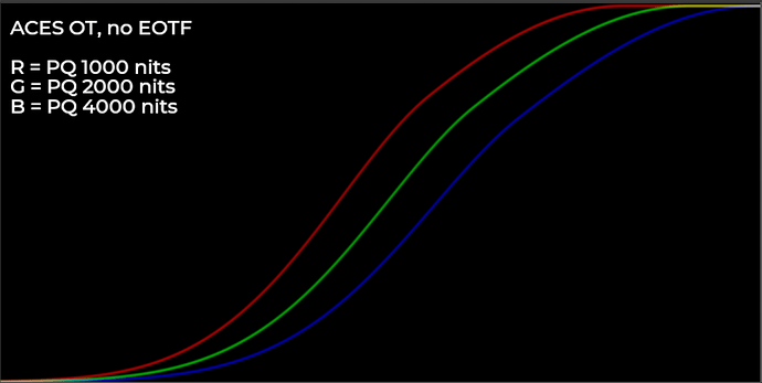
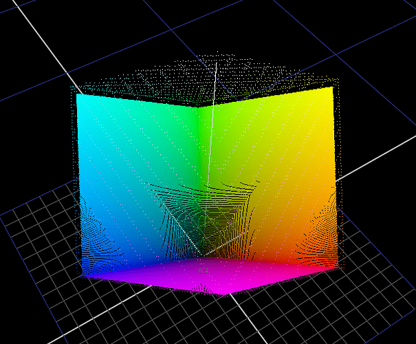
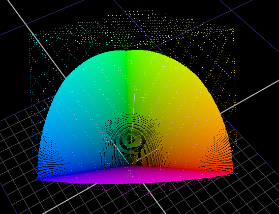
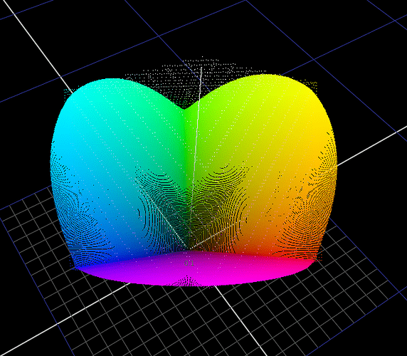
This weekend I’ve spent some time more deeply examining the math of the Michaelis-Menten style compression function that @daniele posted. I have a few useful observations and discoveries which I will share here.
I think it is useful to split apart the compression function into discrete components. I keep going back to the simplicity of my first prototype NaiveDisplayTransform. In that prototype it was very easy to calculate a gamut volume compression as display referred output approaches display maximum, because the “shoulder” compression was an isolated operator. In psuedocode,
norm = max(r,g,b)
shoulder_compress = compress(norm)
factor = 1 - shoulder_compress / norm
factor = pow(factor, bias)
factor is then the factor for the lerp towards 1.0 in the rgb ratios. Super simple, and looks better than the hacks I’ve been doing in my last versions of the OpenDisplayTransform where I am using some power bias of the compressed norm as the factor.
But for this approach to work, shoulder compression must be separated from the other components of the compression.
So! I started digging in to the math of Michaelis-Menten. Daniele’s compression curve is a combination of 4 main things:
- A normalization factor (basically a multiply).
- A shoulder compression to accomplish highlight intensity rolloff.
- A power function to adjust contrast and do surround compensation.
- A toe compression to do flare compensation.
Shoulder
The shoulder compression function is the first thing I started digging into. While implementing my Hill-Langmuir sigmoid compression function, I remember reading in the wikipedia article about it that the Hill-Langmuir equation is a special case of a rectangular hyperbola.
In fact, when n=1 in the Hill-Langmuir equation, the function is a rectangular hyperbola. In it’s simplest form a rectangular hyperbola is the function f\left(x\right)=\frac{1}{x}
When n=1 in the Hill-Langmuir equation above f\left(x\right)=\frac{x}{x+1} Does this look familiar? Yes, it’s a “simple Reinhard” compression function, which is a hyperbola that is offset such that it passes through the origin.
What is super super interesting about these curves however, is how they look on a x-log, y-linear plot. Spoiler: It’s a sigmoid!
Here is a desmos plot showing this:
Toe
So what happens in the Hill-Langmuir equation above when n>1? We are increasing the strength of the toe compression. I didn’t understand this until seeing it split apart in Daniele’s compression curve, but the function is a skewed parabola: f\left(x\right)=\frac{x^{2}}{x+a}
I got really fascinated by this function because I’ve never really seen parabolic functions used in image processing before, and they have a number of very interesting qualities:
- Exponential (parabolic?) increase in compression as the x value approaches the vertex of the parabola.
- Pretty much linear beyond a certain distance from the vertex.
Parabolic Compression Function
So I spent a few days reading about and playing around with Conic Sections and Parabolas, which I haven’t really investigated since highschool many years ago. One super interesting form of this function is as follows f\left(x\right)=\sqrt{2cx+\left(j^{2}-1\right)x^{2}}, where j is the eccentricity and c is the slope.
Depending on the eccentricity, it smoothly transitions form an ellipse to a parabola, to a hyperbola. Pretty crazy! 
Then I got to thinking… (Can you tell I’m really good at getting side-tracked?). Maybe this parabolic function could work really well as a compression function. Back in the gamut mapping virtual working group, the compression function which I liked the look of the most was actually the log compression function. Something about having a more linearly increasing slope over the compressed area, to distribute compressed values more evenly, helped preserve more tonality in affected regions.
This is the desmos plot of that log function
Of course the problem was that there was no closed-form solution for solving for the y=1 intersection (at least not that I could find at the time).
So I spent a little while investigating if there could be a way to create a parabolic compression function which operated in a similar way. It took me a while but I figured out the math to do it. I’ll link desmos plots of my process below in case anyone is interested in this stupidly nerdy stuff:
And finally, in simplified form, with solution for intersection constraint:
f\left(x\right)=\left\{x\ge t:\ c\sqrt{x-t+\frac{c^{2}}{4}}-c\sqrt{\frac{c^{2}}{4}}+t\right\}
where c is the calculated scale factor based on some constraint coordinate which the function must pass through: c=\frac{\left(1-t\right)}{\sqrt{\left(l-t\right)-\left(1-t\right)}}, l is the x coordinate at y=1 that the compression function must pass through, and t is the threshold at which compression starts.
I literally just figured this out so I haven’t really tested it yet, but I’m super curious to see how it works for gamut mapping distance compression.
As usual here it is as a nuke node as well:
CompressParabolic.nk (2.7 KB)
I’ll stop rambling about nerd stuff now. Just wanted to share some of the things I’ve been up to in case anyone is interested or finds this useful! 

 Couldn’t have done that a year ago!)