Output Transform Tone Scale

A few points:

  1. If any value escapes the destination gamut volume, the result is device dependent unless specifically engineered otherwise. This is a fundamental that would need to be addressed in any “management” system.
  2. Baking in something to address Kelvin would also likely affect skin, and few like Rat Piss yellow skin.

In the end, it seems that fundamentals need to be focused on. Here is some good fire, as folks seem to get obsessed with device dependent digital RGB gaudy yellow.

I don’t know if anybody is “obsessed with… yellow”!

Personally my issue with the appearance of fire in unmodified chromaticity linear renderings is that it seems to take on a slightly salmon pinkish tone, which doesn’t feel like fire to me. Although I admit that it could be a learned preference.

1 Like

There is a critical piece of the puzzle being overlooked here, though.

In terms of fundamentals, I reckon that the “pink” is related to that fundamental.

Question: Is everything that comes out of Baselight chromaticity linear? For example, if in Baselight the DRT is set to ACES 0.7 or ACES 1.0.1 would that be chromaticity linear? Or is it only when the DRT in Baselight is set to Truelight CAM that it is chromaticity linear?

If folks go back and read what Jed has said, it’s pretty clear as to why it is of utmost importance.

People aren’t reading.

Tell you what… and again, Jed and others have said this dozens of times, but I’ll repeat it here yet again.

Take a single pixel mixture and run it through a display linear output.

What does it look like? If you manipulate display light in Photoshop, is anyone actually expecting that it magically skews or bends to something other than what the display light mixture is, by default?

Separate creative desires from basic foundational ideas.

Dumb Question #2: @jedsmith Jed speaks in the OP of a

and also

and @nick speaks of

am I correct in understanding that these are all synonymous?

Dumb Question #3 follows from that. Are the hyperbolic and Siragusano that @jedsmith posted here also chromaticity-preserving tone scales?

@Derek: Dumb questions are my favorite because they force explicit definitions, clarifications, and encourage common ground in understanding. Thanks for asking!

First let’s try to define what “chromaticity linear” actually means, because it is a term that believe I made up to try to describe a characteristic. In my understanding, “chromaticity linear” refers to a transformation which moves chromaticities only along a straight line between the original chromaticity and the neutral axis of the colorspace.

Note that I am not using the word “hue” here, because this has nothing to do with nonlinear perception of color in the human visual system.

I don’t believe this is true. Baselight has different display rendering transforms available. TCAM I believe is mostly “chromaticity linear” within the visible spectrum of colors. The ARRI and ACES renderings are not “chromaticity linear” because the chromaticities do not travel along a straight line, as your Planckian Locus sweep above shows pretty clearly.

“ratio preserving tone curve” and “chromaticity-preserving tone scale” mean the same thing. It refers to a compression of input intensity values into a smaller range, which does not change chromaticities in a nonlinear way as a byproduct of that transformation. A chromaticity-linear transform might change the chromaticities as a byproduct, but only in a straight line towards the achromatic axis.

These compression curves are just compression curves. Whether they are chromaticity-preserving or not depends on how they are applied. If you apply the curve directly to input scene-linear RGB values, they will not be chromaticity preserving. If you do something like this, they will be:

vec3 rgb = INPUT_RGB
float norm = max(rgb.x, rgb.y, rgb.z)
float compressed_norm = compress(norm) // some compression function
vec3 out_rgb = (rgb / norm) * compressed_norm

Here’s a little sketch showing the difference a couple test images and the PiecewiseHyperbolic compression curve I posted before.
chromaticity-preserving_vs_per-channel_planckian-locus.nk (222.8 KB)
Using this test image that I like:

This is what the per-channel intensity compression curve looks like on a 1931 chromaticity plot:

This is what the chromaticity preserving method outlined in the code above looks like:

And for interest, here’s a comparison of a chromaticity-preserving and per-channel plot of the Planckian locus looks like. The one bending towards yellow is the per-channel version:
screenshot_2021-05-21_14-49-13

Hope it helps.

5 Likes

@jedsmith yes it helps tremendously, thank you. I love how you are able to take complex brain-busting concepts and explain them in simple terms. That is truly a gift.

One more dumb questions (#4):
Is it the case that when the RRT “look” is added to a chromaticity-preserving tone map that the “salmon” color kelvin will look sunshine yellow again?

This was my hope with the ARRI ALF-2 look that I applied in Baselight over the T-CAM DRT. In my test above it does have that nice yellow sun color. That’s promising. However, I’m seeing an issue with green on the ALF-2. The following is an exposure sweep of renders of colored spheres, similar to the one from @ChrisBrejon except these are in ACEScg primaries, rather than sRGB primaries.

Both the T-CAM and T-CAM with the ALF look appear to be chromaticity-preserving, in that they are not shifting from 12 colors to the “notorious 6.” However, the pure green on the top row is clipping something awful. Looks to me like it’s a gamut problem. If I apply @jedsmith gamutCompress.nk to it, set to “ACEScg from Filmlight E-gamut” it’s not perfect (the green diffuse color is brighter than the spec), but certainly a ton better.

In the end, it seems like there is a tradeoff between having a 1 to 1 with material colors (chromaticity-preserving) or having a 1 to 1 with light color. If that is the case, then I guess the question is what would be more important to artists? However, I’m still hoping that with the right “look” (and maybe some gamut voodoo) artists can have both. Is that hope realistic?

Yes. In my development work I have implemented an inverse for the OpenDRT. With this it is trivial to construct an LMT which, when applied before the display transform, exactly matches the ACES output transform (within the limits of the display encoding of course). I believe this approach is more flexible and will allow more creative freedom than the way things are done currently.

1 Like

I have been working a bit on parameterization since my last post, Trying to figure out a robust and simple model for how the different parameters change with different display outputs.

I have settled on a set of parameters which I think are pretty simple and work pretty well, even for HDR.
screenshot_2021-05-22_13-52-28

  • Lp - Peak display luminance in nits. Used for HDR output, when peak white and peak luminance of the inverse EOTF container might not match. For example for ST-2084 PQ rendering, Lp will be 10,000 and Lw might be some other value.
  • Lw - White luminance in nits. In SDR, Lw and Lp would probably be equal.
  • Lg - Grey luminance in nits.
  • Contrast - a constrained contrast control which pivots around the output middle grey value.
  • Surround - an unconstrained power function adjustment for surround luminance adjustment.
  • Toe - a parabolic toe compression for flare compensation.

There is then a layer of calculations which calculates static values based on the above parameter set:
screenshot_2021-05-22_13-57-49

  • p = Final power function parameter. Equal to Contrast * Surround
  • grey - Input → Output grey mapping. Output grey value equal to Lg / Lp
  • w - Input exposure adjustment. Calculates a scale factor such that input grey maps to output grey through the compression functions.
  • w_hdr - Boost input exposure by some amount when Lw > 1000 nits. I have calculated it here as max(1,pow(Lw/1000,0.1)), but this could be creatively adjusted. (This paramete is not pictured above, as it is included in the scale).
  • h - Simple linear model which adjusts output domain scale such that clip occurs at some finite input domain value. This varies with Lw: 0.048*Lw/1000+1.037 is what I came up with, but it could be adjusted creatively.
  • scale - Final input and output domain scales:
    scale.x = w * w_hdr,
    scale.y = Lw / Lp * h

Here are two compression functions using this parameterization. The first is based on @daniele 's formulation, but with some modifications so that input domain scale happens first and output domain scale happens last:
Tonemap_ToeLast_v1.1.nk (3.3 KB)

The second is a simpler version of my piecewise hyperbolic compression function with the white intersection constraint removed, because it is no longer necessary with this parameterization.
Tonemap_PiecewiseHyperbolic_v3.nk (4.0 KB)

Here are a few plots showing the behavior of the HDR curve with varying values of Lw, through the piecewise hyperbolic curve. The input is an exponential input ramp, ranging from 5 stops below 0.18 to 12 stops above 0.18. This lets us see a log-ranging x-axis in the plot. Note that in these plots I have removed the output scale which normalizes Lw to the correct position in the PQ container, so that we can see peak white at 1.0 for all curves in order to compare them effectively.


1 Like

Unless I misunderstood what you are trying to say, isn’t it already something we can do (and do) with ACES? It is a scenario that was deemed highly non-desirable. The inverse + forward approach is subject to many issues WRT precision, e.g. quantization, especially with a LUT implementation, and performance, i.e. double-transformation cost. From an architecture standpoint, @daniele’s proposal here, inscribed in the “put-your-own-DRT” paradigm, is much cleaner.

Cool stuff! Quick question though as I haven’t loaded your Nuke scripts: What is the Y-axis red line here? Might be worth plotting 0 on the X-axis also.

What I said above was an incomplete thought. Let me try to elaborate.

I agree with you one hundred percent that it is highly undesirable to build LMTs through the inverse of the display transform. The fact that this is required with the current ACES system is a huge problem that absolutely needs to be resolved. Daniele’s proposal is fanstastic and absolutely the best path forward in my opinion.

All I mean to say above is that it is possible to form an LMT that exactly matches the current ACES Output Transforms, if it were desired.

By this I mean to say that if we were to have a chromaticity-linear display transform with minimal look and a robust inverse, it would be better to build LMTs “on top of” than the current ACES Output Transform. Hopefully this makes sense.

I am 1,000% in favor of an output transform agnostic system, but as it has been said before, I believe we still need a good looking default for the more novice users.

The red line is display-linear 1.0. Hopefully it made sense what I typed above. Let me summarize:

  • The X-Axis of the plot is log-ranging, with a minimum on the far left edge of 5 stops below 0.18, and a maximum on the far right edge of 12 stops above 0.18. The X-Axis origin is not pictured.
  • In these plots I have removed the output domain scale which place white at the correct position for the PQ Inverse EOTF, so that we can more easily compare what is happening to the curve at different values of Lw.
1 Like

I spent a little time today porting some Nuke tools to DCTL and Blinkscript.

Here are the two tonemapping functions from my last post:
EOTF.dctl (4.0 KB)
Tonemap_PiecewiseHyperbolic.dctl (4.2 KB)
Tonemap_ToeLast.dctl (3.7 KB)

I’ve also added blinkscript versions in my git repo here:

Hope it’s useful as a better reference implementation, and for to help people less familiar with Nuke to experiment and play around.

2 Likes

Further Simplification of the Parameter Model

I spent some time doing further work on the parameter model. My goal is to figure out a simple elegant behavior for the curve control parameters in terms of display luminance Lw, in order to create a model that smoothly transitions from SDR to HDR.

Previously I had a control w for boosting exposure with HDR peak luminance like @daniele mentioned in one of the previous meetings. I wondered if this idea could be extended to a simple model for changing grey nit level Lg based on peak white luminance Lw. Maybe something that would work across all values of Lw from 100 nits to 4000 nits.

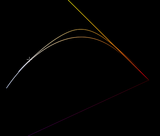
I gathered some sample values, looked at the behavior, and used the desmos regression solver to come up with a simple log function which models it pretty well. This could of course be altered depending on rendering or aesthetic preferences.
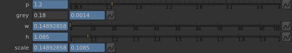
L_{g}=14.4+1.436\ \ln\left(\frac{L_{w}}{1000}\right)

The result sets the middle grey value based on Lw pretty effectively.

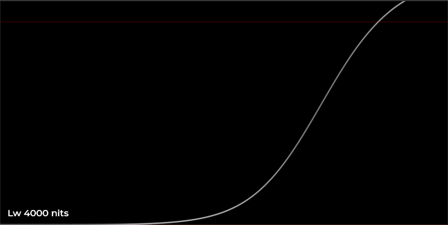
Doing the same thing for the toe flare/glare compensation control: t_{0}=\frac{1}{L_{w}} seems to be a very good fit to the observed behavior of how the amount of toe compensation should be reduced as peak luminance increases.

All of this should be further refined and validated with testing of course, but the behavior seems to work quite well with the limited consumer-level display devices which I have at my disposal.

Experiment Time

Most LCD computer monitors these days can output 250 nits or more. Yet if we are calibrating to Rec.709, we set the luminance to 100 nits.

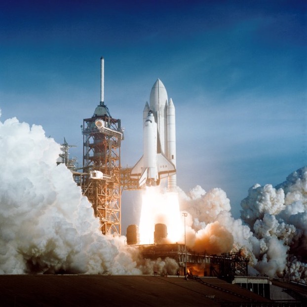
For a long time I’ve wondered if it were possible and what it would look like to render an image for proper display on a monitor with a higher nit level. Using the model described above I decided to finally do just such an experiment. I’ll share the results here because I think they are pretty interesting and do a good job of showing the visual difference between hdr and sdr in a relative way.

Experiment Summary

I have two computer monitors:

  • HP Dreamcolor Z27x G2
  • DELL U2713HM

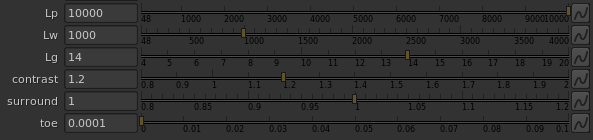
I set my Dell to be 100 nits and my HP to be 250 nits. Using OpenDRT_v0.0.81b3, I rendered one image using Lw = 100 nits, and one using Lw = 250 nits and put them on their respective monitors.

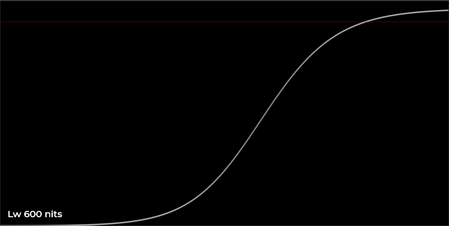
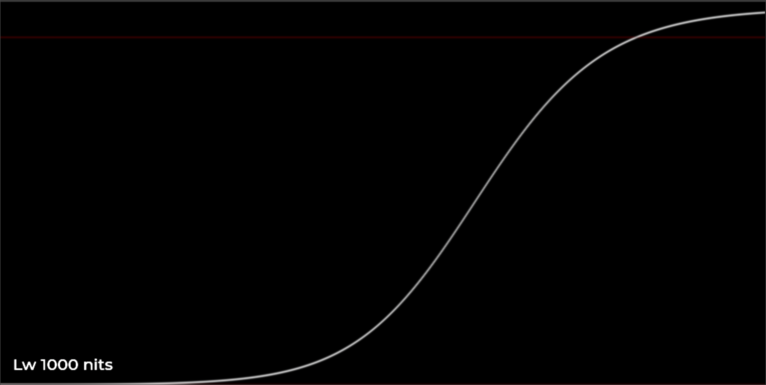
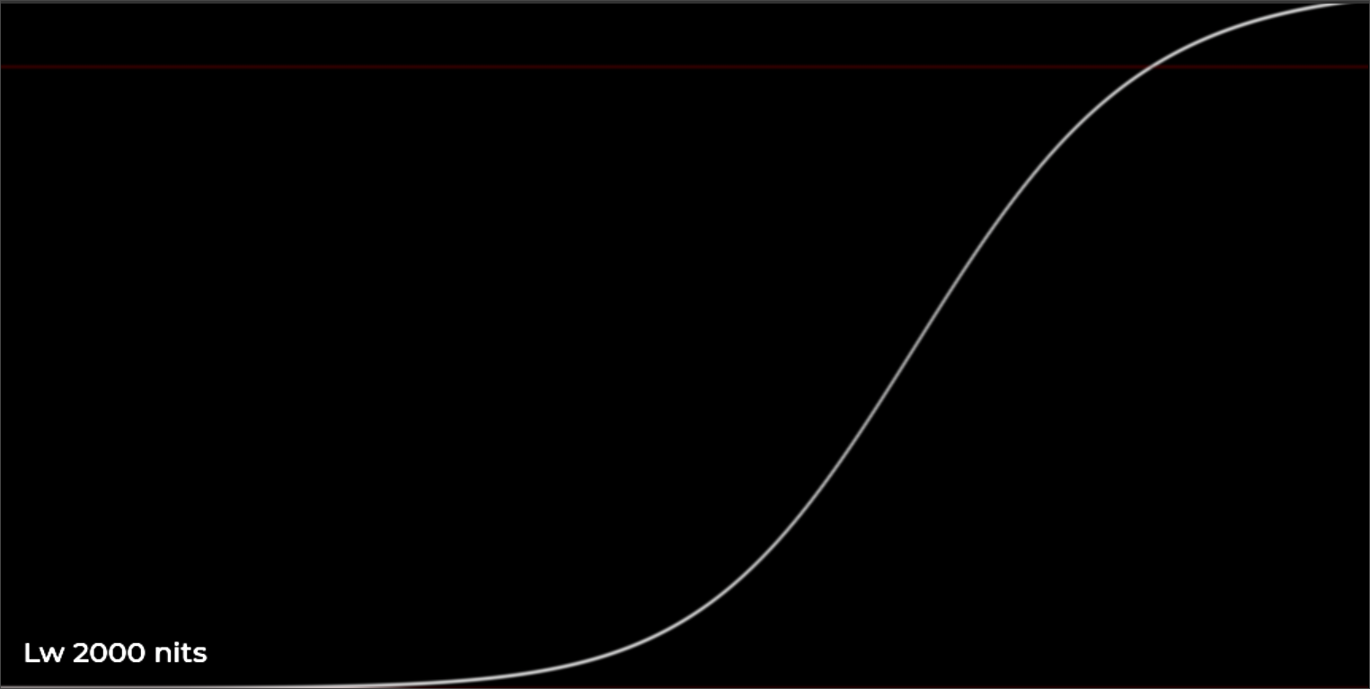
I was surprised that their appearance actually looked pretty similar, after my eyes adjusted. The 250 nit version had more range and clarity in the highlights and shadows, and the 100 nit version looked a bit more dull and compressed. Once my eyes adapted to each image though, their appearance was very similar. We can do a variation of this comparison using only one SDR monitor with the luminance cranked up as far as it will go. By rendering one image with a peak white of some value, say 250 nit or 600 nit, and the other image with a 100 nit white luminance, but a peak luminance matching the 250 nit or 600 nit output (this can be achieved by overriding the Lp setting in the OpenDRT node).

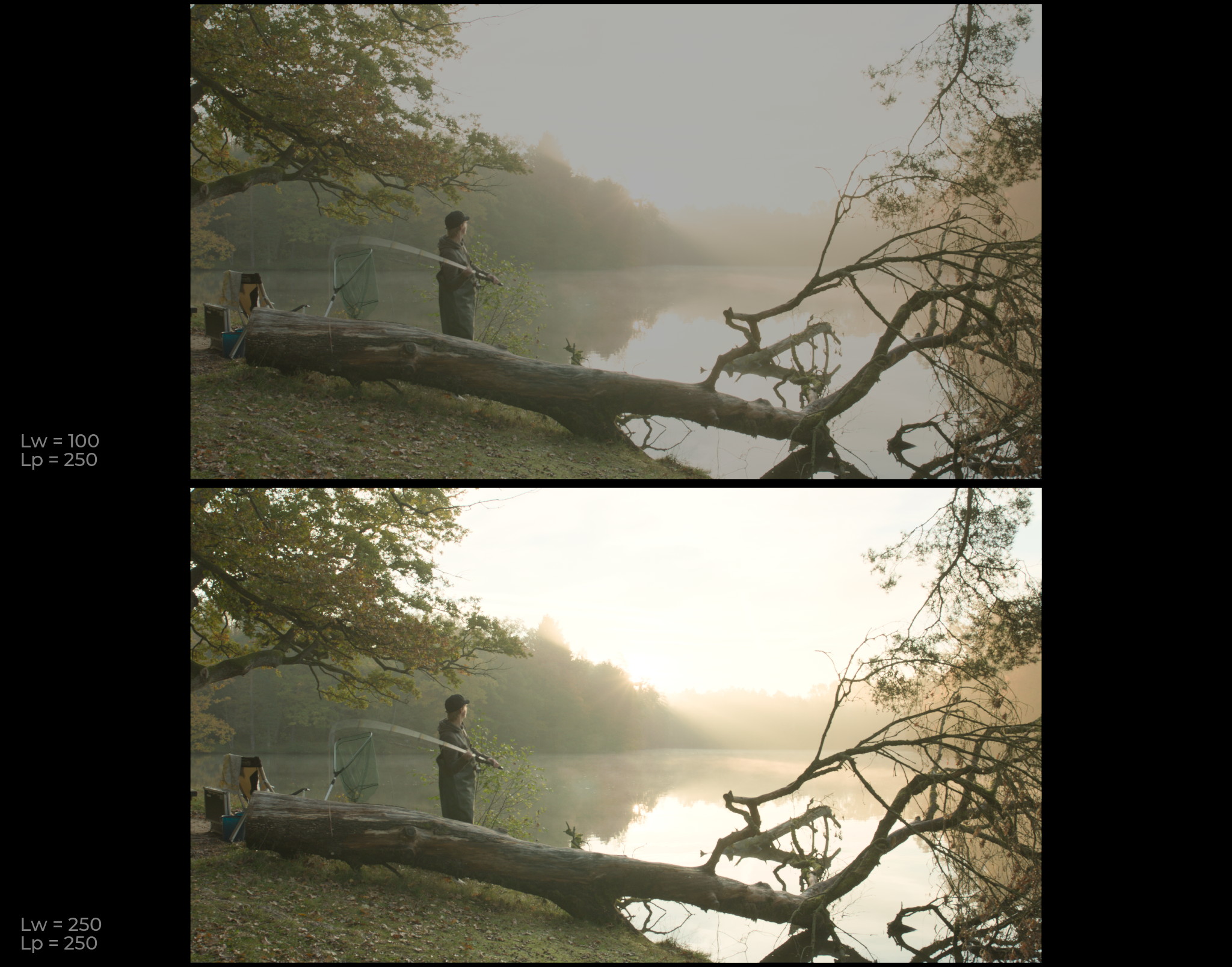
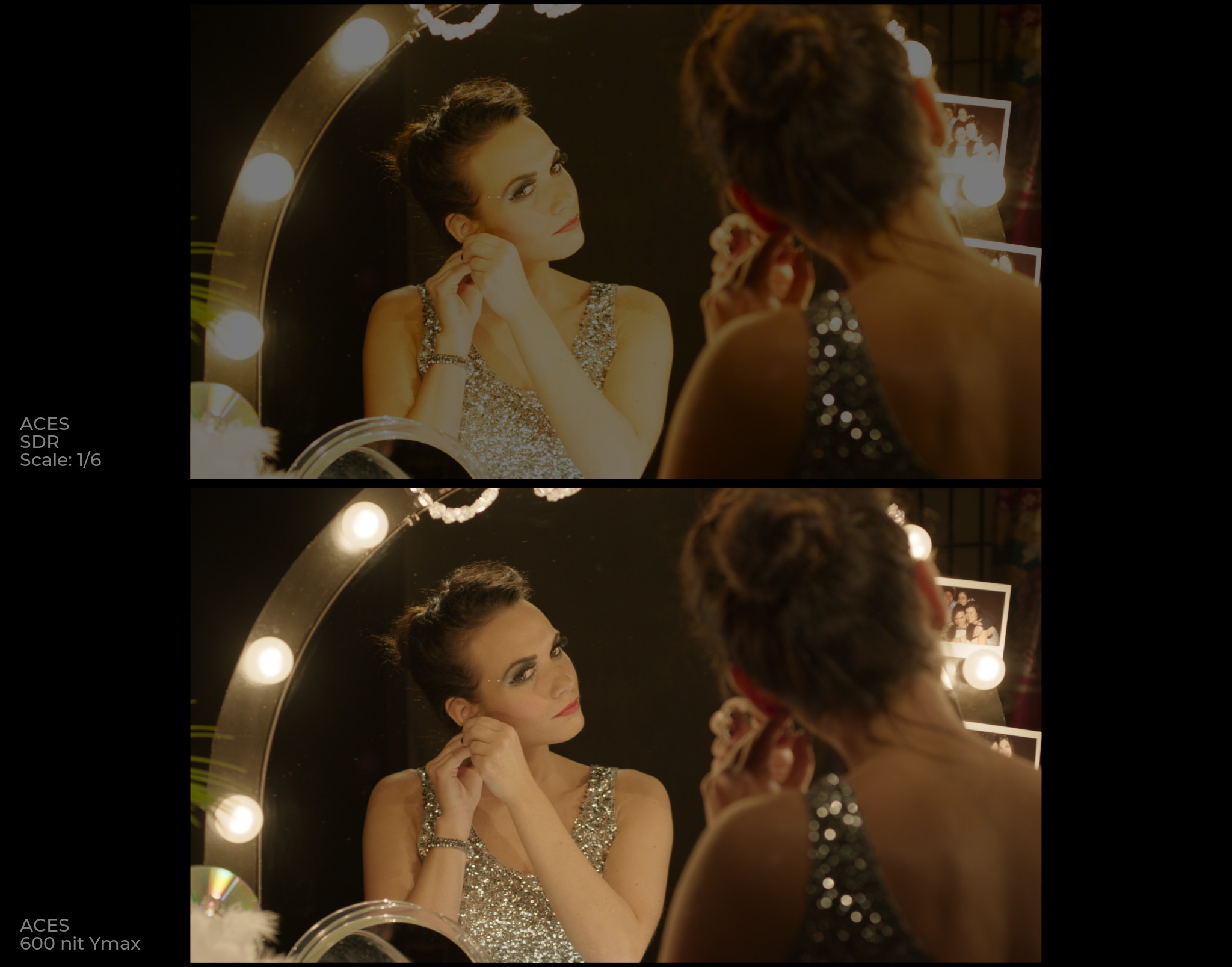
I’ll include a couple of comparison images below. To view them, crank up your monitor brightness as high as it will go and view the images full screen with no UI visible, and do the comparison in a dark room with the lights off. Also if you have something like a piece of black foam-core to cover the image you are not viewing, it will help you get a more accurate perception.

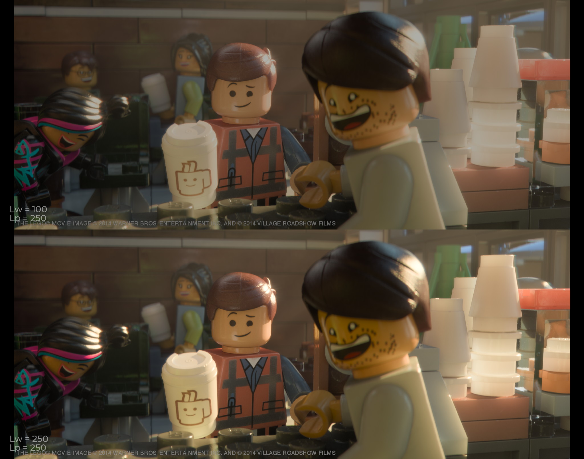
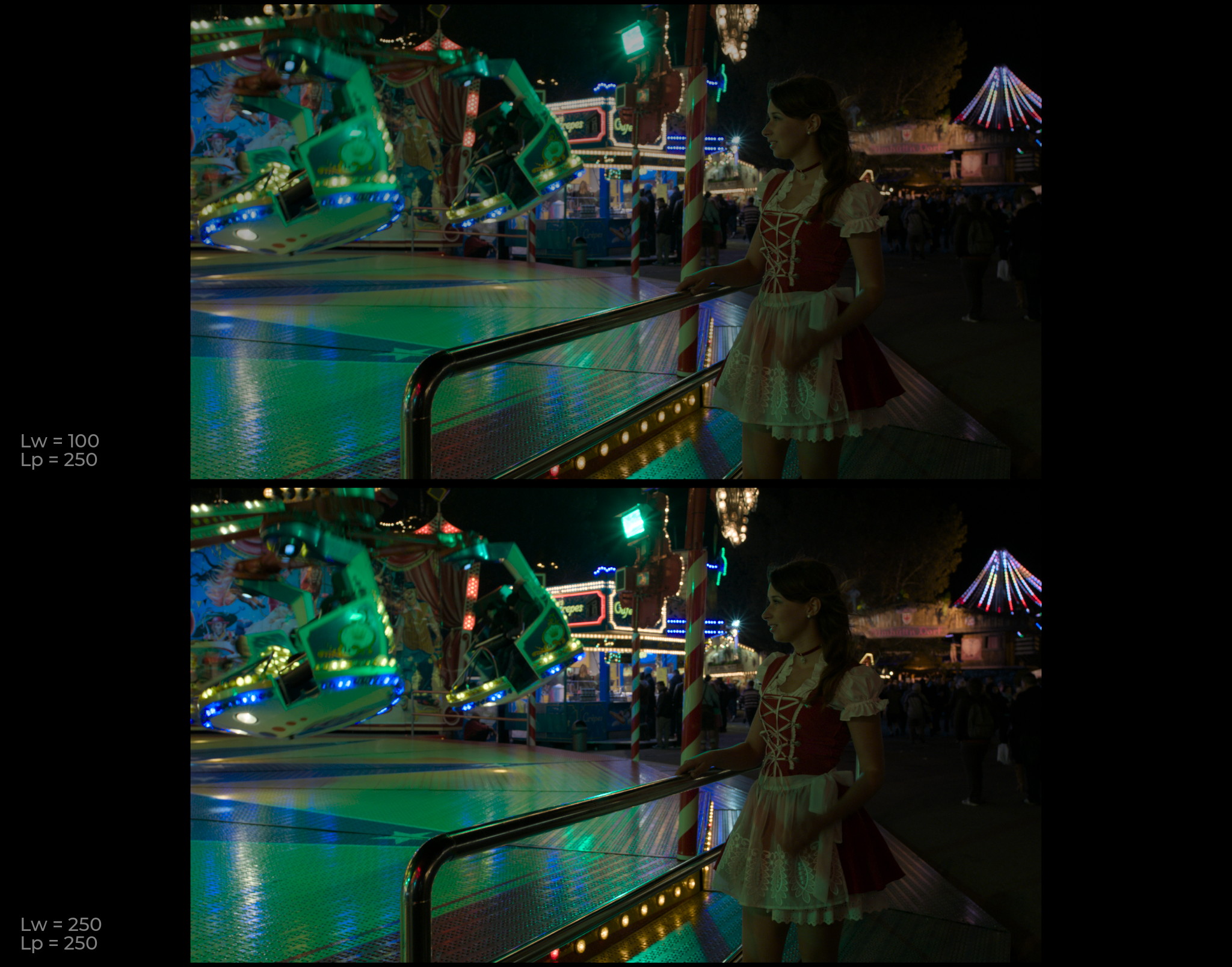
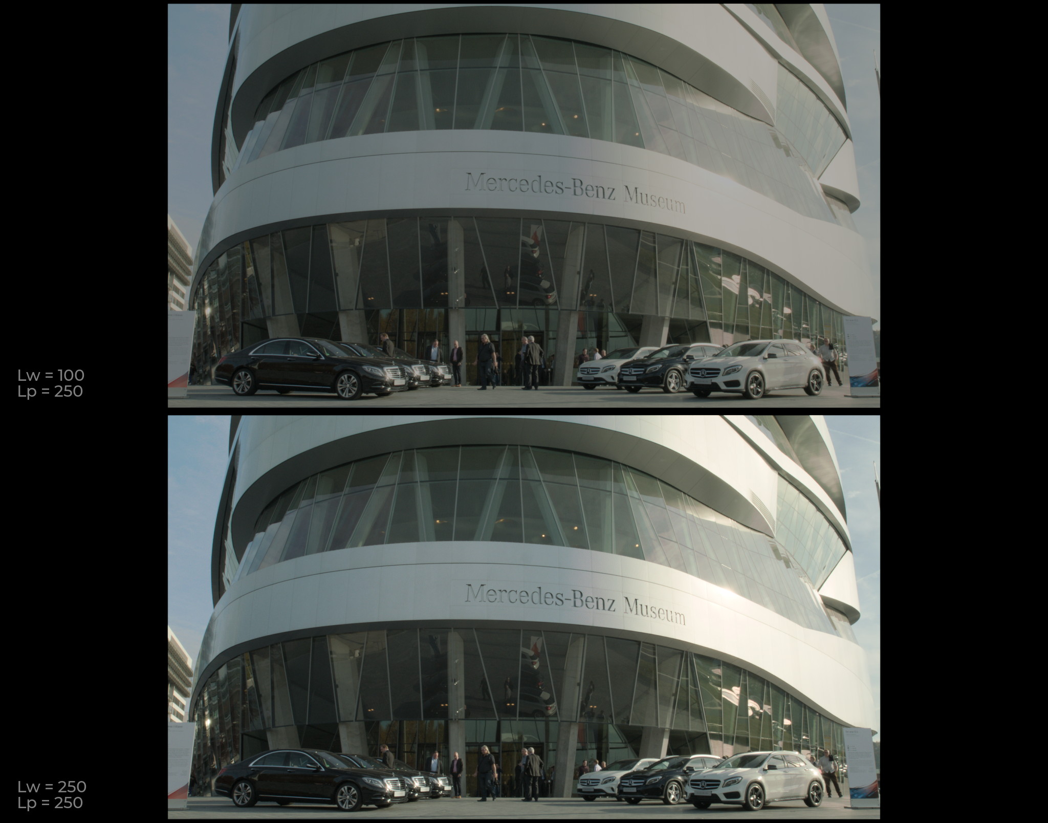
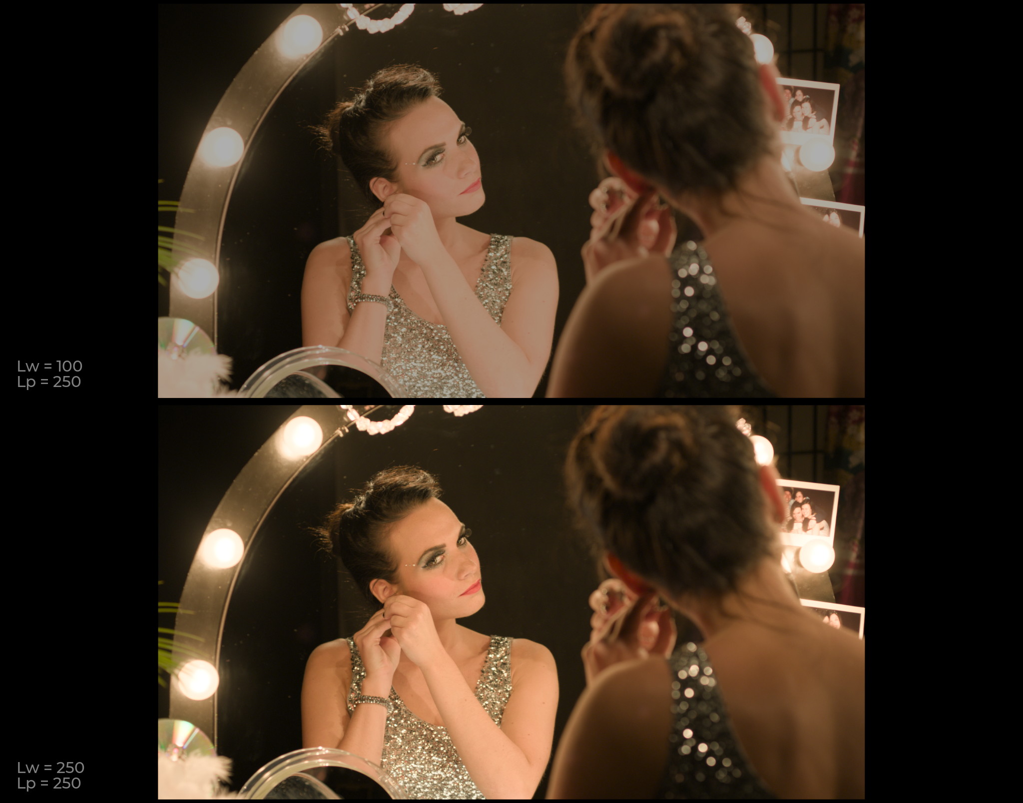
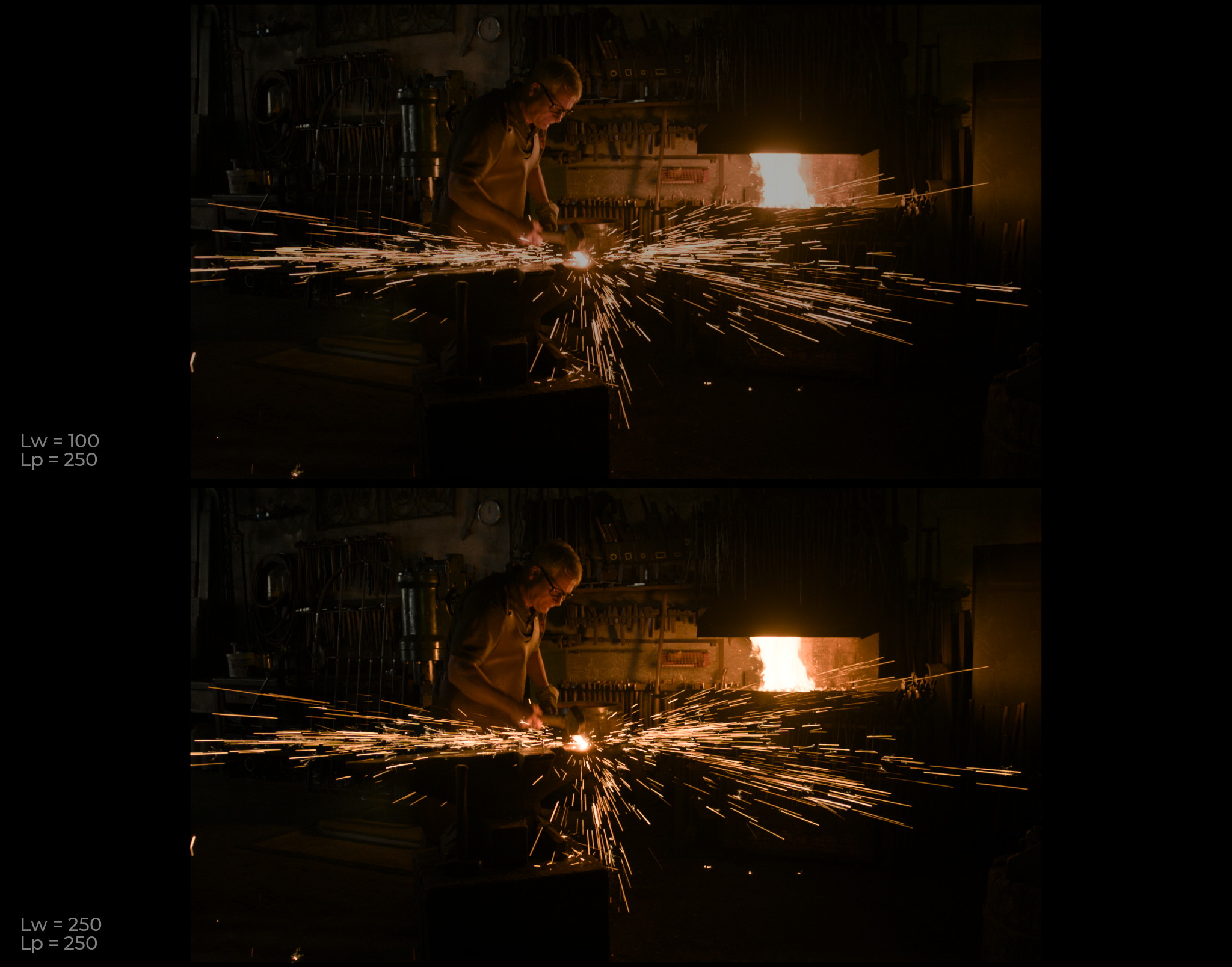
On the top is an image scaled to simulate a 100 nit output on a 250 nit monitor: Lw = 100, Lp = 250.
On the bottom is the same image rendered at the full 250 nits: Lw = 250, Lp = 250.


I’ve uploaded more of these test images here:
https://mega.nz/folder/zmQFGYIQ#QBi5RkfFfaCdV4rfc06_hA

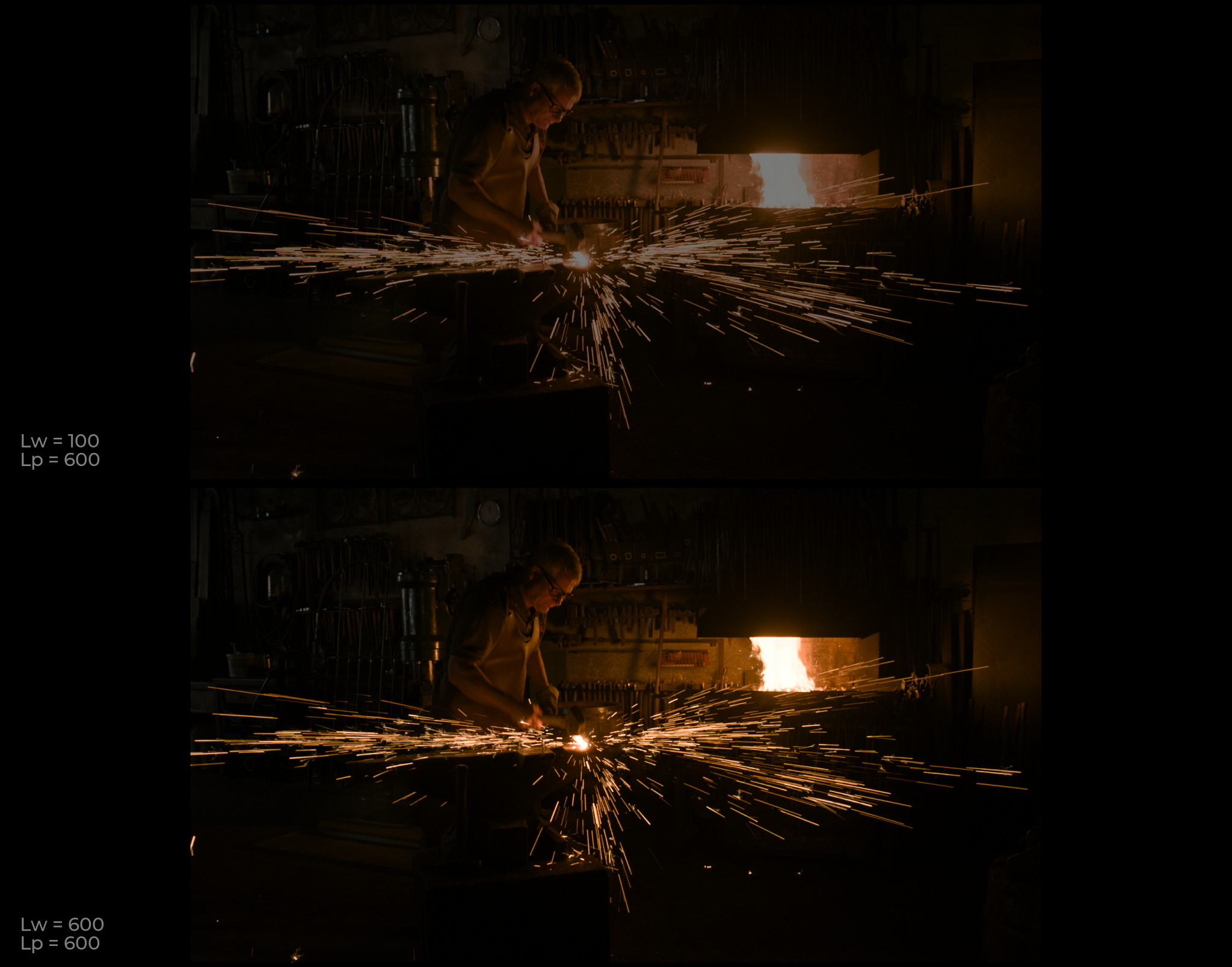
The same experiment could be performed to compare a 600 nit rendering to a 100 nit rendering, though maybe less precise without access to a proper HDR display.


And all the same images but vs.600 nit available here:
https://mega.nz/folder/XzZHiaTI#CT3VbT94pg-BHxEkafJlGg

And here is the nuke script I used to generate all these test images.
opendrt_100nit_vs_hdr.nk (193.2 KB)

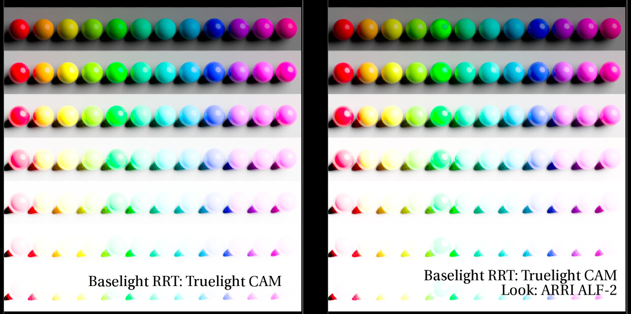
The source images are from the ODT VWG, the Gamut Mapping VWG and the VMLab Stuttgart HDR Test Images, and a few beautiful CG Renders by @ChrisBrejon (Hopefully he doesn’t mind me using them here).

With the increase in “VESA Display HDR 400” monitors, I think this experiment is particularly relevant today.

I’m somewhat confident I’ve set all of this up correctly, but if any of you smart people see any errors feel free to point them out!

2 Likes

I went ahead and ran out the same image set through the ACES Output Transform modified to output 600 nit HDR in a BT.1886 container, compared with SDR, same as above.
https://mega.nz/folder/e2ongI6a#wkjlR1_y4JMcGbcsoqrObw

Just to make it clear what the images are:

  • Bottom image is display linear result of 600 nit HDR display render transform, without any peak display luminance normalization (e.g., 600 nit luminance is mapped to 1.0 in display linear, instead of 600 / 10,000 like it would need to be if dumping into a ST-2084 container)
  • Top image is display linear result of a 100 nit SDR display render transform, scaled so that display linear 1.0 matches 100 nits on a 600 nit display (e.g., display linear 1.0 equals 100 / 600)

This shows the “rough relative appearance difference” between the “look” of the hdr rendering, and the sdr rendering, in a way that can be seen on a normal computer monitor.

I think these images do a good job of showing the HDR / SDR appearance match issues with the per-channel approach.

And the nuke script that generated the images if anyone wants to play:
aces_100nit_vs_hdr.nk (237 KB)

1 Like

That’s very interesting Jed.

Having little experience with HDR (unfortunately), I think these examples help a lot ! I agree that these images show clearly that the hue shifts/skews will be dependent of the RGB (per-channel) lookup “compression”.

It reminded me of this paper (originally shared by Kevin Wheatley). Quoting the conclusion :

The maxRGB variation is the only implementation, out of the five presented in this article and summarized in Table 5, that accomplishes both objectives [restricting luminance and minimizing hue variance].

And this makes me wonder how this could be solved in the current ACES Output Transform (for the possible prototype’s evaluation). If I recall correctly, it has been stated a couple of times that this would be very tricky to correct for.

Because if it is device/display dependent, doesn’t it beat the whole idea of color management ?

Best,
Chris

Hello,

I don’t think your comparison is really valid, the transformation chain you applied on the top image never occurs in practice, you are effectively doing this:

Inverse EOTF(OutputTransform_{Abridged}(RGB) \cdot \cfrac{100}{600})

In a proper image formation chain, the signal is never scaled the way you expressed your transformation chain. Trying to model the display peak luminance effect on appearance like that is not correct, if anything scaling should occur at the very end. It is a by-product of the display calibration characteristics, not something happening somewhere middle of the display rendering transform.

Cheers,

Thomas

Unless I’m missing something, I’m not entirely sure this is true. For example in the ACES Output Transform this type of scaling is exactly what happens to the display linear light code values before it is put into the ST-2084 PQ Inverse EOTF container. But maybe I don’t understand what you mean.

Just to confirm I understand what you are saying, you are suggesting to scale display light after the inverse eotf has been applied?

In fact maybe I don’t understand what you are saying at all. Maybe you can you do me a favor and outline exactly how you would approach previewing the “rough relative appearance difference” between 600 nit hdr and sdr on an sdr display?

This transformation never occurs for SDR and for HDR it is scaled by Y_{max}, to be exact, in ACES, it is linCV * (Ymax - Ymin) + Ymin. However, here you are not scaling by Y_{max} but a factor of it, which people will never see in practice on a SDR display. With that in mind, and given your images have been encoded for SDR exhibition, I don’t think that your modeling is really appropriate to convey relative appearance.

Well, I don’t think you can in any meaningful way, the inverse is totally possible though!

Cheers,

Thomas